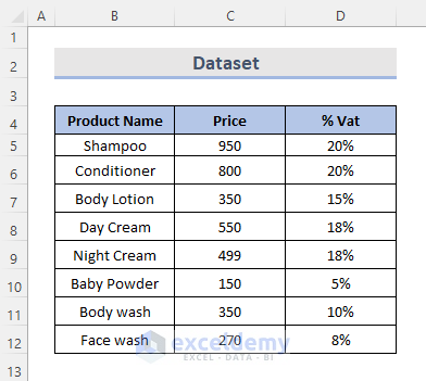
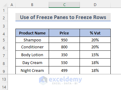
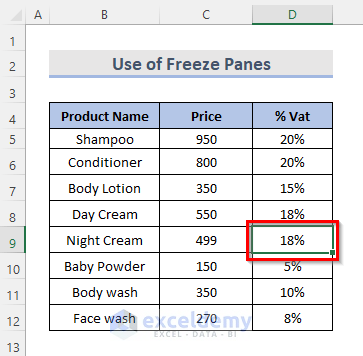
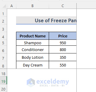
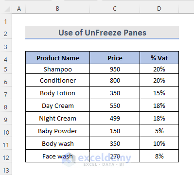
To Freeze multiple panes in Excel, we are using the dataset below. The dataset contains some product names in column B and their price in column C, as well as the product’s percentage of value-added tax (VAT).
Method 1 – Freeze Multiple Rows in Excel
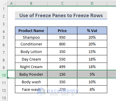
Let’s freeze the rows up to row 10.
Steps:
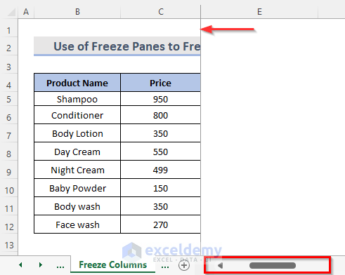
- Select the rows you want to freeze from the list below. We want to freeze rows 1 to 9 in our case, so we chose row 10.
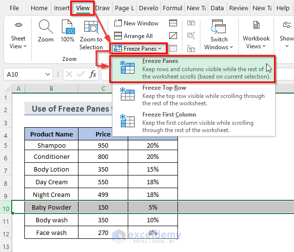
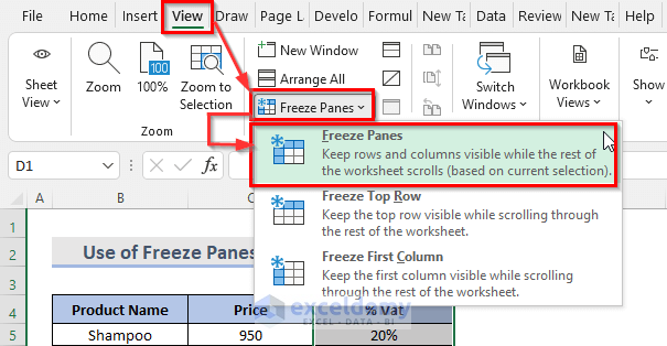
- Select the View tab on the ribbon.
- Choose Freeze Panes from the Freeze Panes drop-down menu of the window group.
- The rows will lock in place.
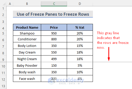
- We can scroll down the worksheet to see the frozen rows at the top while going down.
Read More: How to Freeze Rows and Columns at the Same Time in Excel
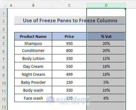
Method 2 -Lock Multiple Columns in Excel
Let’s freeze column B and column C.
STEPS:
- Select the column behind those we want to freeze. So, we will select column D.
- On the ribbon, select the View tab.
- In the Freeze Panes drop-down menu in the Window group, choose the Freeze Panes option.
- We can see the gray line which indicates that the columns are now locked.
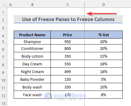
- By scrolling right, we can view the frozen data columns.
Note that this also froze column A, since you have to freeze columns starting from the first one.
Method 3 – Freeze Both Rows and Columns Together in Excel
Steps:
- Select a cell that is below the rows and right to the columns we want to freeze. We selected cell D9 to freeze the product name and price up to Day Cream.
- Select the View tab from the ribbon.
- In the window group, from the Freeze Panes drop-down menu, choose Freeze Panes.
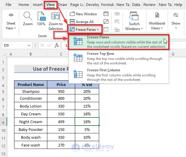
- This freezes just before cell D9 both vertically and horizontally, with two lines to note the frozen row and column.
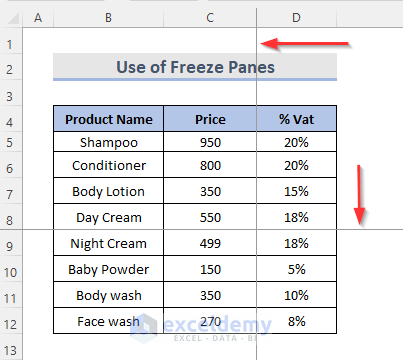
- You can scroll along the worksheet to see the frozen rows and columns.
Related Content: Keyboard Shortcut to Freeze Panes in Excel
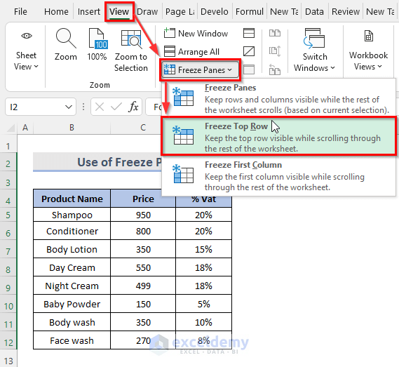
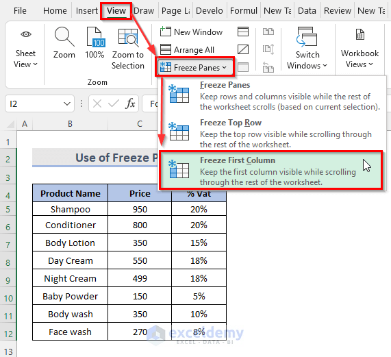
Method 4 – Lock the Top Row and the First Column
Steps:
- Go to the View tab on the ribbon in the sheet.
- To lock the top rows, choose the Freeze Top Row option from the Freeze Panes drop-down menu in the Window group of the View tab.
- To lock the first column, choose the Freeze First Column option from the Freeze Panes drop-down selection in the Window category of the navigation pane to lock the first column.
Read More: How to Freeze Top Row and First Column in Excel
Unfreeze Multiple Panes in Excel
Steps:
- Check if your dataset contains frozen rows or columns.
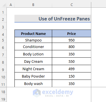
- Go to the View tab from the ribbon.
- Choose Unfreeze Panes from the Freeze Panes drop-down menu under the Window category to unlock the data.
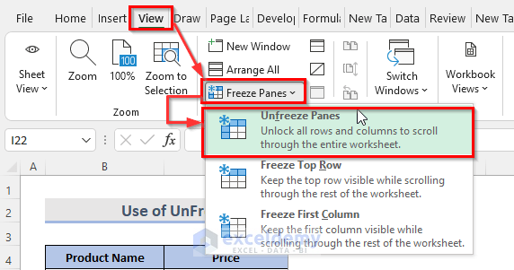
- Finally, just clicking on the Unfreeze Panes will unlock all the rows and columns.
Freeze Panes Aren’t Operating Properly
If the Freeze Panes button in our worksheet isn’t working, it’s probably because of one of the following:
- You’re editing a cell instead of the sheet itself. Press the Enter or Esc key to go out of a cell.
- Your spreadsheet has been password-protected. Unprotect the worksheet before freezing the rows or columns.
Download the Practice Workbook
You can download the workbook and practice these methods.
Related Articles
- How to Unfreeze Rows and Columns in Excel
- How to Apply Custom Freeze Panes in Excel
- Excel Freeze Panes Not Working
- How to Freeze Panes with VBA in Excel
<< Go Back to Freeze Panes | Learn Excel
Get FREE Advanced Excel Exercises with Solutions!
