Method 1 – Using the Freeze Panes Command to Freeze the Top 3 Rows
Steps:
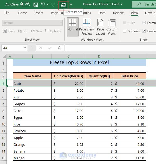
- Select the 4th row.
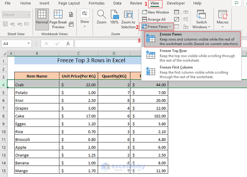
- Go to the View tab and click on Freeze Panes from the Window ribbon.
The Freeze Panes menu will appear. There are three options in the Freeze Panes menu.
- Click on the Freeze Panes option from the dropdown menu of the Freeze Panes of the View tab.
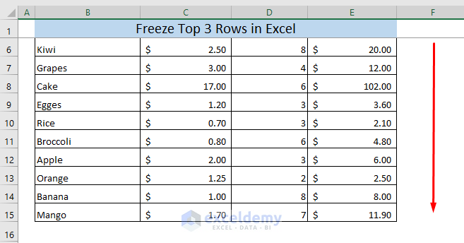
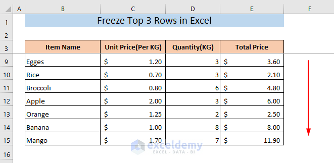
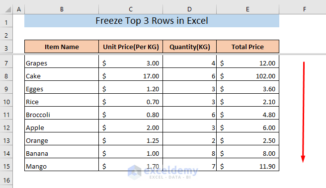
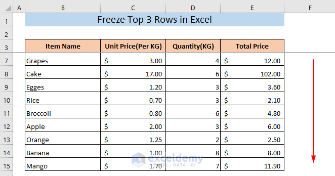
It will freeze the top 3 rows of your worksheet. If you scroll down, the top 3 rows are always visible.
Read More: How to Freeze Top Row in Excel
Method 2 – Freezing the Top 3 Rows with a Split Window
Steps:
- Select the 4th row.
- Go to the View tab and click on the Split icon.
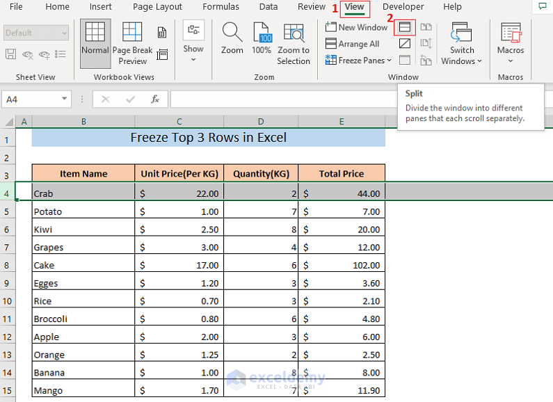
It will freeze the top 3 rows of your worksheet. If you scroll down, you will find the top 3 rows are always visible.
Read More: How to Freeze Top Two Rows in Excel
Method 3 – Applying an Excel Freeze Button to Fix the Top 3 Rows
Steps:
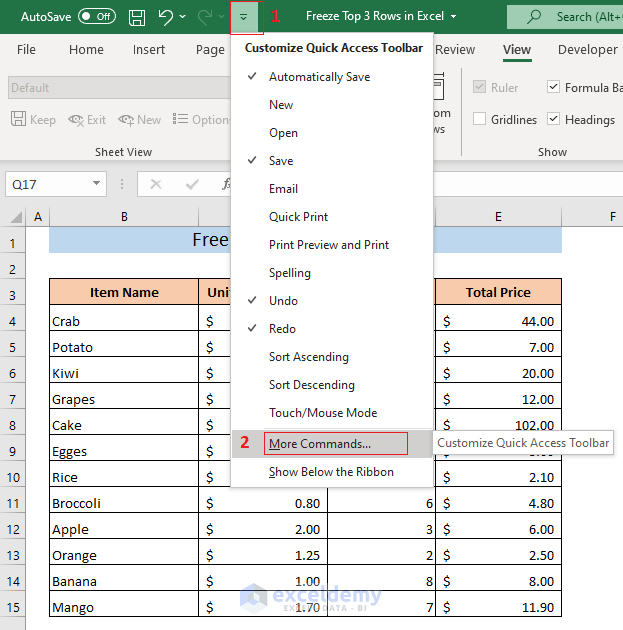
- Click on the drop-down icon from the top bar of the Excel files.
- It will open a drop-down menu.
- Select More Commands from this menu.
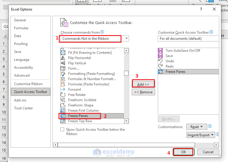
- The Quick Access Toolbar tab of the Excel Options window will appear.
- Select Choose Not in the Ribbon in the Choose Command from box.
- Select Freeze Panes and click Add. It will add the Freeze Panes option in the right box.
- Click OK.
You will see a Freeze Panes icon in the top bar of your Excel file.
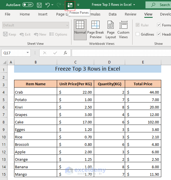
- Select the 4th row and click on the Freeze Panes icon.
It will freeze the top 3 rows of your worksheet. If you scroll down, you will find the top 3 rows are always visible.
Read More: How to Freeze Columns in Excel
Things to Remember
Freeze and split panes cannot be used at the same time. Only one of the two options is available.
Only the rows at the top of your selected row will be frozen. You must select the 4th row to freeze the top 3 rows.
Download the Practice Workbook
Related Articles
- How to Freeze 2 Columns in Excel
- How to Freeze First 3 Columns in Excel
- Unfreeze Rows in Excel
- How to Unfreeze Columns in Excel
- How to Freeze Random Selection in Excel
- How to Lock Cells in Excel When Scrolling
- How to Unlock Cells in Excel When Scrolling
- How to Lock Rows in Excel When Scrolling
<< Go Back to Freeze Panes | Learn Excel
Get FREE Advanced Excel Exercises with Solutions!
