Unfreeze Rows in Excel (3 Quick Ways)

When you work with a large dataset, you may find it challenging to scroll through multiple rows and columns. Fortunately, Excel offers the option to freeze rows and columns to keep certain information visible while scrolling down through the rest of the worksheet. Also, it is important to know the system to unfreeze the rows in Excel.

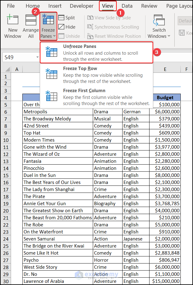
As a newbie in Excel, you may face difficulties in unfreezing the rows. In this article, we are going to show you the ways to unfreeze rows in Excel. We have used the Freeze Panes option, the keyboard shortcut, and a short VBA code to unfreeze the panes. The below overview image shows one of the methods to unfreeze rows using the Unfreeze Panes option.

Unfreeze Rows in Excel: 3 Quick Ways

As a beginner in Excel, you may find it difficult to freeze the rows and columns. To do this, we have taken a dataset from the IMDB Movies Database where lots of movie-related data are stored. When you freeze the rows, you need to unfreeze the rows in Excel. We have discussed the methods to do it.

There are no frozen rows in our above dataset. So, we have to apply any of the methods to freeze rows in Excel. Here, we have used the Freeze Panes option.

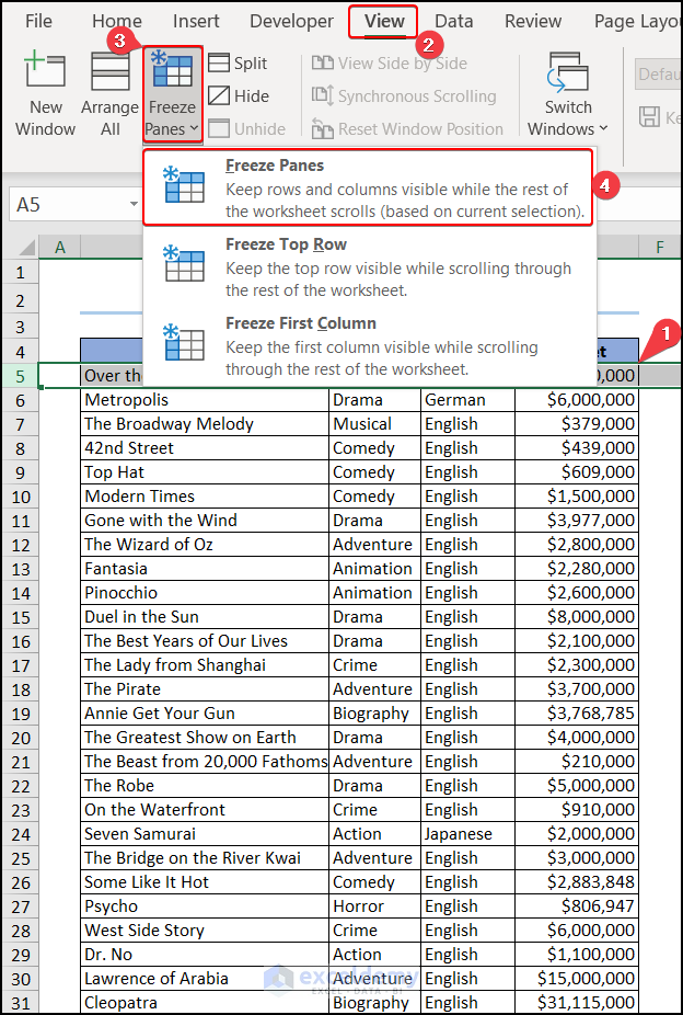
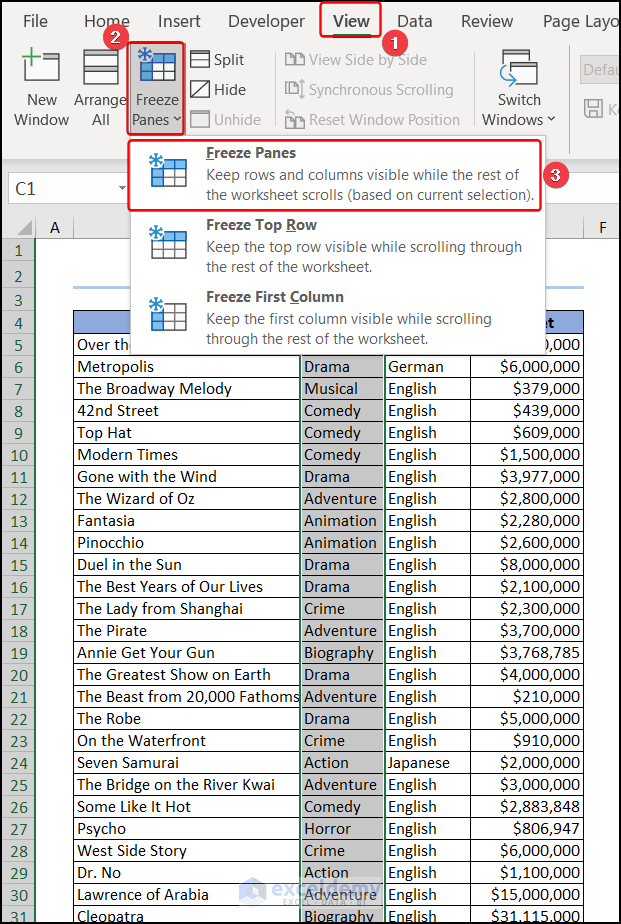
• First, you need to freeze the rows. To freeze your column header, you need to select the entire row just beneath the header row. Then move to the View tab >> select Freeze Panes from the Window group >> pick Freeze Panes.

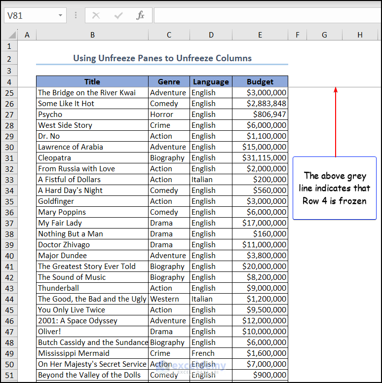
A grey line appears. This line indicates that the above rows are frozen. When you scroll down the mouse, the data will be moved upward, leaving the header intact as Row 4 is frozen.

Not to mention, we have used the Microsoft 365 version. You may use any other version at your convenience.

1. Using Unfreeze Panes Option from the View Tab

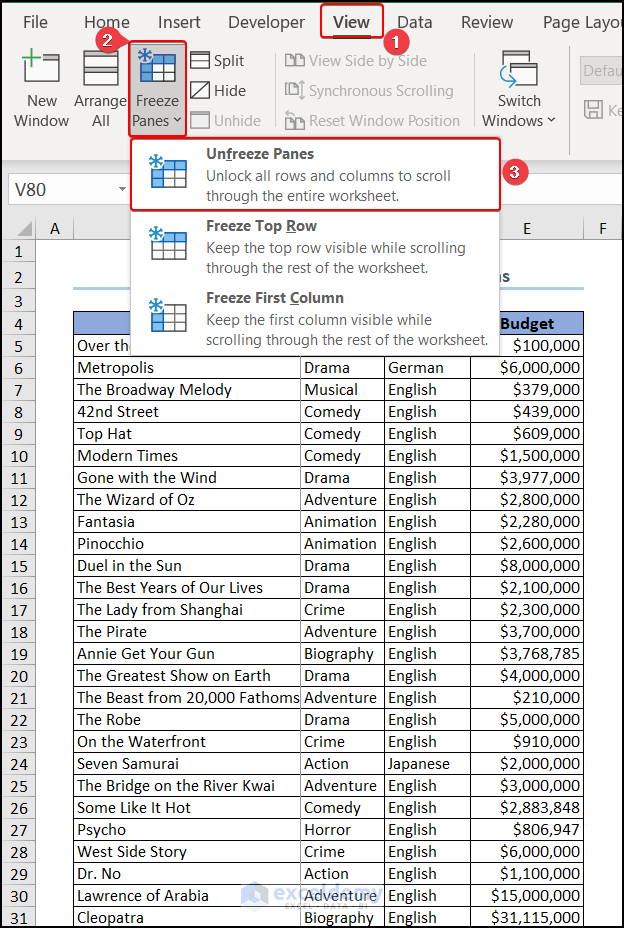
When you need to unfreeze the rows, you need to hover over the View tab >> choose Freeze Panes from the Window group >> pick Unfreeze Panes.

Your frozen rows will be unfrozen quite easily, as you can see in the below image.

2. Using keyboard Shortcut to Unfreeze Rows

We can also use the keyboard shortcut to unfreeze rows in Excel. It is quite an easy and quick process, so it saves a lot of time.

• Firstly, press the ALT+W key on your keyboard.
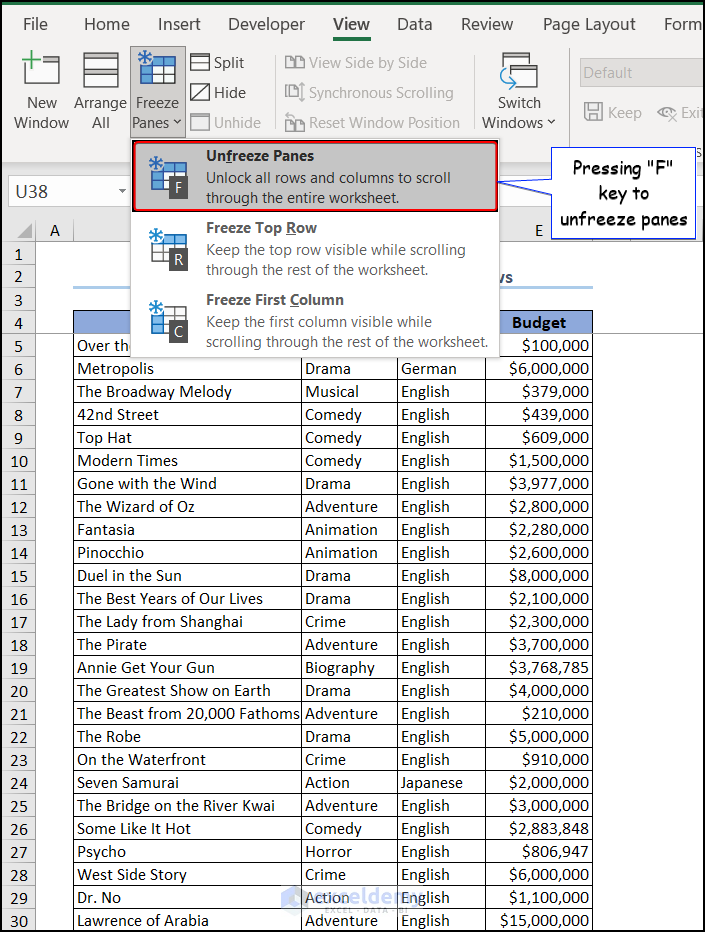
• Eventually, a prompt will appear in the ribbon tab like the below image. Press the “F” key on your keyboard to open the Freeze Panes options from the Window group.

• Next, press the “F” key again to unfreeze the panes.

So, the final keyboard shortcut is ALT + W + F + F.

Finally, you have unfrozen the rows that you locked before.

Read More: Keyboard Shortcut to Freeze Panes in Excel

Similar Readings

• How to Lock Cells in Excel When Scrolling
• How to Unlock Cells in Excel When Scrolling
• How to Freeze Top Row in Excel
• How to Lock Rows in Excel When Scrolling
• How to Freeze Top Two Rows in Excel
• How to Freeze Top 3 Rows in Excel

3. Applying VBA to Unfreeze Rows in Excel

You can also use the VBA code to unfreeze rows. The VBA automates your dataset and makes your work fast.

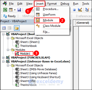
• To use VBA for unfreezing rows, first go to the Developer tab >> choose Visual Basic.

• The Visual Basic Editor window appears. Navigate the Insert tab >> select Module >> Module1.

• Write the following VBA code to unfreeze.

Sub UnfreezeRows()
ActiveWindow.FreezePanes = False
End Sub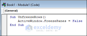

In the above code, we have used the ActiveWindow.FreezePanes property. This property set to False indicates that if there is any freeze pane in the active window, then it will unfreeze as soon as we make it False.

Finally, run the code with the F5 key, and the freeze panes will be gone.

How to Unfreeze Columns in Excel

You can freeze your desired column. When you have a lot of columns in your dataset, you may need to freeze a specific column. In that case, if you scroll the other columns sidewise, the selected columns will be locked in the first place.

To freeze a column, select the column that is after your header column. In our dataset, we have selected column C. Then navigate to the View tab >> choose Freeze Panes from the Window group >> select Freeze Panes.

• A grey line appears that indicates column C is frozen.

• Now, if you want to unfreeze the columns then again go to the View tab >> pick Freeze Panes and select the Unfreeze Panes option from there.

Finally, the freezing columns will disappear, as shown in the below image.

Read More: How to Unfreeze Columns in Excel

Frequently Asked Questions

• How do we unfreeze Excel without losing data?

You may also select File>Info>Manage Workbook>Recover Unsaved Workbooks when the Excel applications open to see whether your workbook is among those listed there. If you locate it, choose it, click “Open,” and then save it once more.

• How do we freeze 3 rows in Excel?

Choose the row underneath the row or rows you wish to freeze. (Select Row 5 if you want to freeze Rows 1–4). Click Freeze Panes > Freeze Panes under the View tab.

• How do we unfreeze rows and columns in numbers?

Choose Freeze Header Rows or Freeze Header Columns from the pop-up options located underneath Headers & Footer to freeze the header rows and columns. Deselecting Freeze Header Rows or Freeze Header Columns will remove the freeze condition.

• How do we lock specific columns in Excel?

Go to the Protection tab, uncheck the Locked option, and click Ok. Now select only the cells, columns, or rows that you want to protect. Right-click and choose Format cells again. Go to the Protection tab, check the Locked option, and click Ok.

Things to Remember

• Ensure that you have selected the correct row to unfreeze.
• If you are not sure enough about which rows need to be unfrozen then just use the “Unfreeze Panes” option to unfreeze rows.
• When you unfreeze rows, the frozen rows will become unfrozen and scrollable along with the rest of the data. So, it is important to keep cautious while unfreezing.

Download Practice Workbook

Download the following practice workbook. It will help you understand the topic more clearly.

Conclusion

So, these are some easy and quick processes to unfreeze rows in Excel. We hope this method helps you understand how to unfreeze clearly. If you have any queries or need any kind of help with an Excel-related problem, feel free to inform us through emails or comments. Our expertise will try to solve your problem. Thanks for your patience in reading the article.

Related Articles

• How to Freeze 2 Columns in Excel
• How to Freeze First 3 Columns in Excel
• How to Freeze Multiple Panes in Excel
• How to Freeze Top Row and First Column in Excel
• How to Freeze Rows and Columns at the Same Time in Excel 
• How to Apply Custom Freeze Panes in Excel
• How to Freeze Panes with VBA in Excel 
• How to Freeze 2 Columns in Excel
• Excel Freeze Panes Not Working
• How to Unfreeze Rows and Columns in Excel