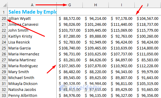
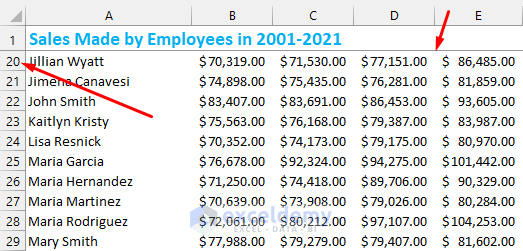
This article shows you how to freeze top rows in Excel in 4 different ways. You can freeze the top row in just two clicks by following one of the methods. The following picture highlights the results.
How to Freeze the Top Row in Excel: 4 Easy Ways
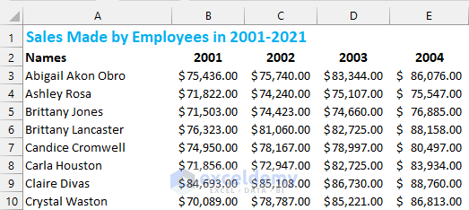
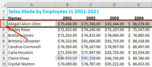
Suppose we want to display this description even if we scroll down through the data. We can apply the following methods to do that easily.
Method 1 – Freeze the Top Row Using the Quick Freeze Tool
Steps
- Select File and go to Options.
- Select Quick Access Toolbar.
- Scroll down the list of popular commands to find Freeze Panes and select it.
- Click on the Add button. You can see the Freeze Panes command has been added to the Quick Access Toolbar list. Make sure it is added to all documents.
- Hit the OK button.

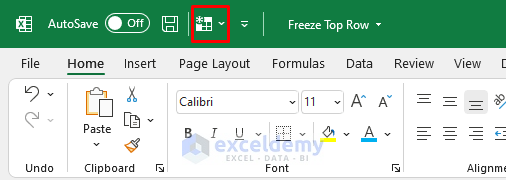
- You will see the Freeze Panes command as a quick access tool as follows.
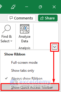
- If you don’t find it there, you need to activate Show Quick Access Toolbar.
- Select the Freeze Panes quick access tool and choose Freeze Top Row.
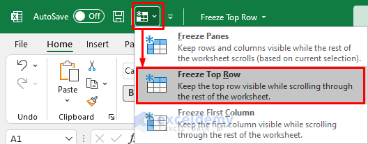
- You will see a solid line below the top row. Scroll down to see if the top row is frozen and always visible.
Read More: How to Freeze Top Two Rows in Excel
Method 2 – Freeze the Top Row From the Freeze Panes Window
Steps
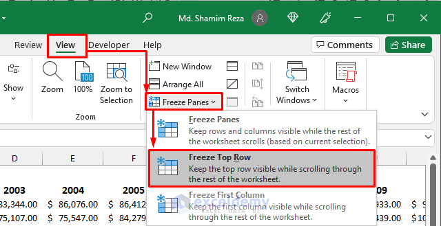
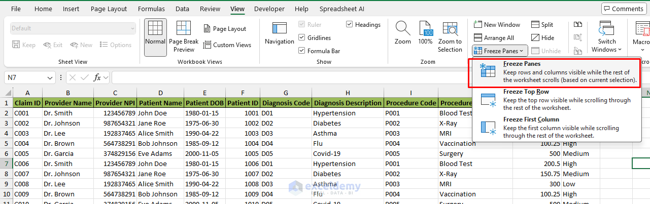
- Go to the View tab.
- Find the Freeze Panes command in the Window group.
- Select the Freeze Top Row command.
Read More: How to Freeze Top 3 Rows in Excel
Method 3 – Freeze Multiple Top Rows in Excel
Steps
- Select the first cell in the row after the rows you want to freeze.
- Click on the row number at the left of the row. The entire row will be selected.
- Choose Freeze Panes instead of Freeze Top Row in the Freeze Panes command tool.
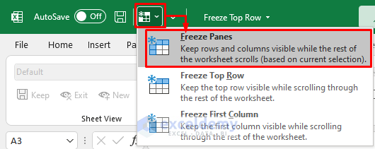
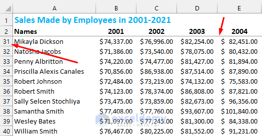
- Scroll down to see if the top rows are frozen.
Read More: How to Freeze Columns in Excel
Method 4 – Freeze the Top Row and the Leftmost Column Together
Steps
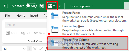
- Choose the Freeze First Column option instead of the Freeze Top Row in the Freeze Panes command.
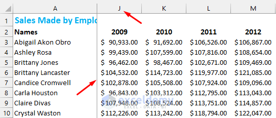
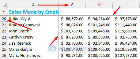
- You will see a solid line at the right of the first column. Scroll horizontally to see that the leftmost column is frozen. To freeze multiple leftmost columns, select the column next to the columns you want to freeze and then choose Freeze Panes.
- If want to freeze the top row and the first column at the same time then the first scrollable cell will be B2.
- Select cell B2 and then select Freeze Panes.
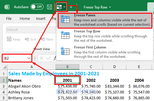
- You will see a solid line below the top row and another one at the right of the first column.
You can freeze multiple top rows and leftmost columns in the same way. All you have to do is just select the first scrollable cell and then select Freeze Panes.
Read More: How to Freeze 2 Columns in Excel
Things to Remember
- You can only freeze the row or rows from the top and column or columns from the left in Excel. Excel doesn’t freeze any middle rows or columns.
- Always select the row or column next to the rows or columns you want to freeze.
Download the Practice Workbook
Related Articles
- How to Freeze First 3 Columns in Excel
- Unfreeze Rows in Excel
- How to Unfreeze Columns in Excel
- How to Freeze Random Selection in Excel
- How to Lock Cells in Excel When Scrolling
- How to Unlock Cells in Excel When Scrolling
- How to Lock Rows in Excel When Scrolling
<< Go Back to Freeze Panes | Learn Excel
Get FREE Advanced Excel Exercises with Solutions!

What year is this from? There is no “Freeze Panes” option in the “Freeze Panes” drop down. There is only “Unfreeze Panes”, “Freeze Top Row” and “Freeze First Column”.
Hello Roy E. McCarthy,
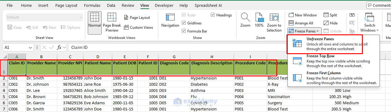
We are using MS Office 365. In Excel, once you freeze any row or column, the option will change to “Unfreeze Panes” instead of showing “Freeze Panes” again. This helps users know that something is already frozen. If you want to freeze or unfreeze rows or columns, you need to select the appropriate option based on your current status.
Before freezing anything:
After freezing first row:
Regards
ExcelDemy