How to Freeze Top Row and First Column in Excel (5 Methods)

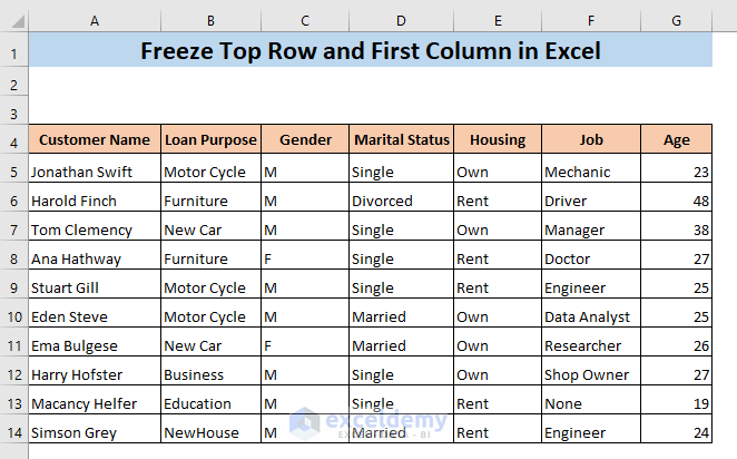
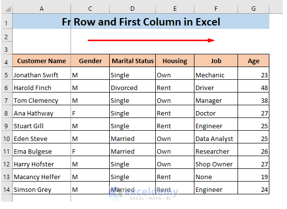
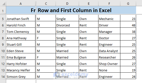
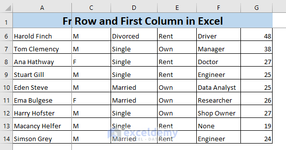
We have the following dataset regarding customer information, where you want to freeze the top row and the first column.

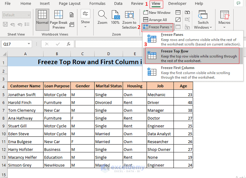
Method 1 – Freezing the Top Row Only

• Go to the View tab and click on Freeze Panes from the Window ribbon.
• The Freeze Panes menu will appear.
• Click on Freeze Top Row.

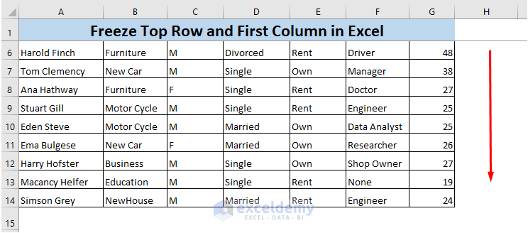
• If you scroll down, the top row will always remain visible.

Read More: How to Freeze Rows and Columns at the Same Time in Excel 

Method 2 – Freezing the First Column Only

• Go to the View tab and click on Freeze Panes from the Window ribbon.
• Select Freeze First Column.

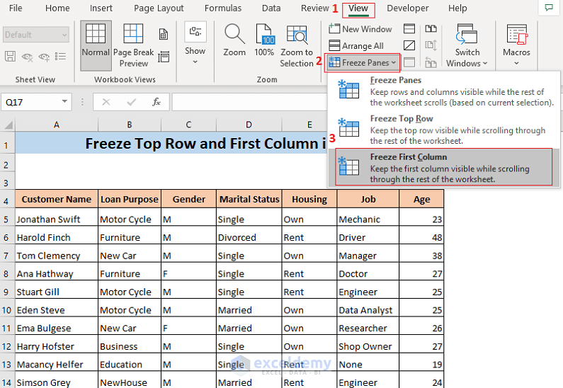
• If you scroll right, the first column will always remain visible.

Read More: Keyboard Shortcut to Freeze Panes in Excel

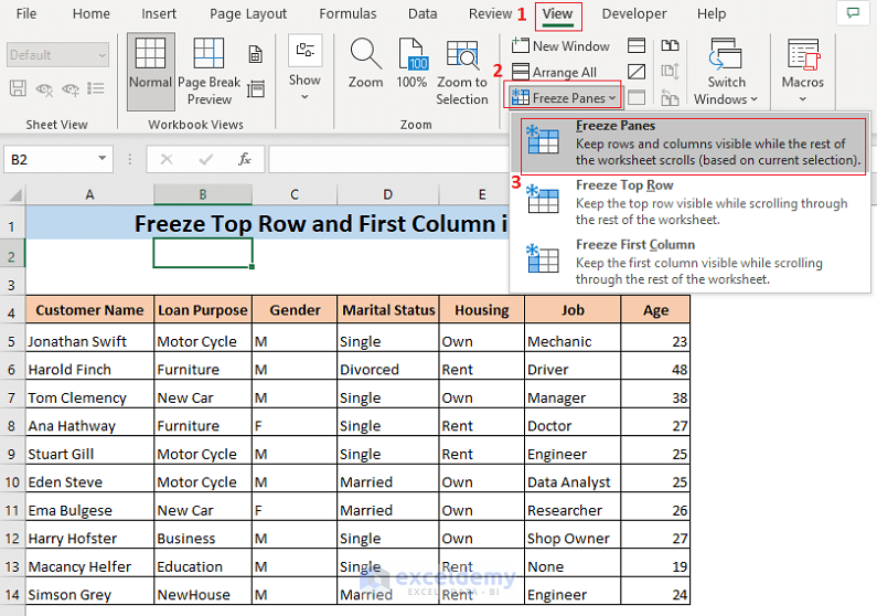
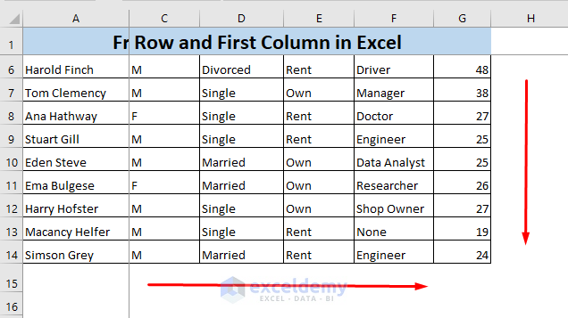
Method 3 – Freezing the Top Row and the First Column Simultaneously in Excel

• Select cell B2.

The reference cell must be exactly below the row and to the right of the column you want to freeze.

• Go to the View tab and click on Freeze Panes from the Window ribbon.
• Select Freeze Panes.

• When you navigate through your worksheet, the top row and the first column will always remain visible.

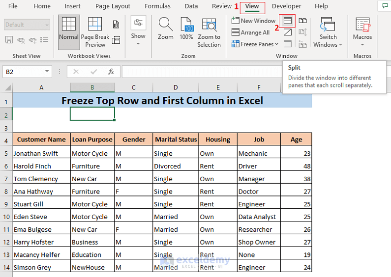
Method 4 – Splitting Panes to Freeze the Top Row and the First Column in Excel

• Select the cell B2

The split cell must be below the row and to the right of the column you want to freeze.

• Go to the View tab and click on the Split icon.

• The top row and the first column of your dataset will be frozen. The data is separated into four windows.

Read More: How to Freeze Multiple Panes in Excel

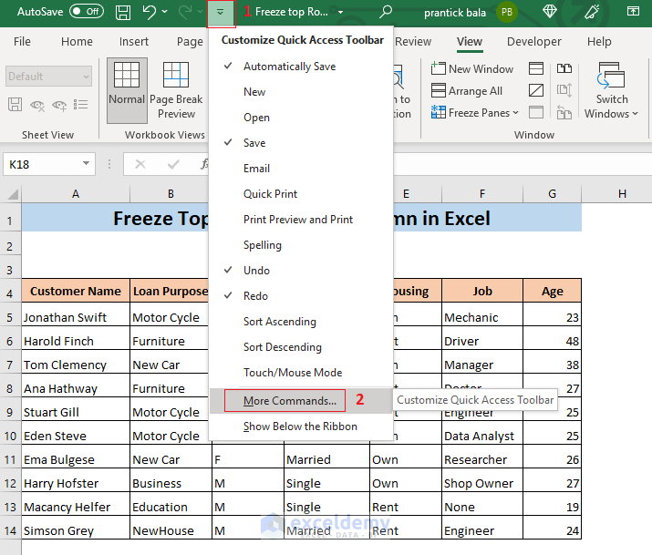
Method 5 – Using the Excel Freeze Pane Button to Fix the Top Row and the First Column

• Click on the drop-down icon from the top bar of the Excel files.
• Select More Commands.

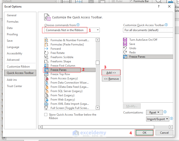
• The Quick Access Toolbar tab of the Excel Options window will appear.
• Select Choose Not in the Ribbon in the Choose Command from box.
• Select Freeze Panes from the list and click on Add.
• This will add the Freeze Panes option to the list on the right.
• Click on OK.

• You will see a Freeze Panes icon in the top bar of your Excel file.

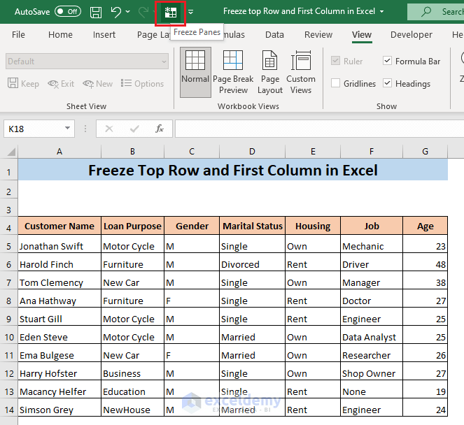
• Select cell B2 and click on the Freeze Panes icon.

Read More: How to Apply Custom Freeze Panes in Excel

Things to Remember

Freeze and split panes cannot be used at the same time.

If you want to freeze rows and columns at the same time, the reference cell must be below the row and to the right of the column, you want to freeze.

Download the Practice Workbook

Related Articles

• How to Unfreeze Rows and Columns in Excel
• Excel Freeze Panes Not Working
• How to Freeze Panes with VBA in Excel 

<< Go Back to Freeze Panes | Learn Excel