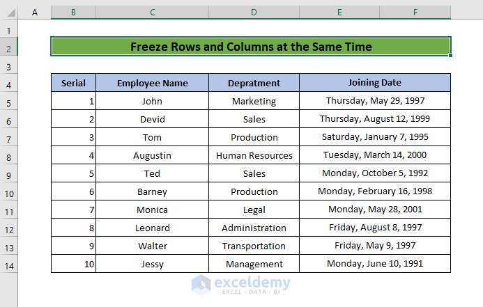
We have an Excel worksheet with information about a company. We’ll freeze the column header and the employee names so they stay on the screen while scrolling.
Method 1 – Using Freeze Panes to Freeze Columns
Steps:
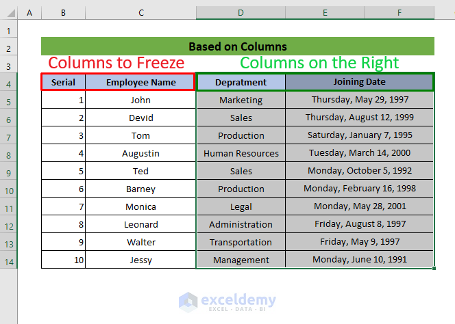
- Since we’re freezing columns up to column C, select the D column.
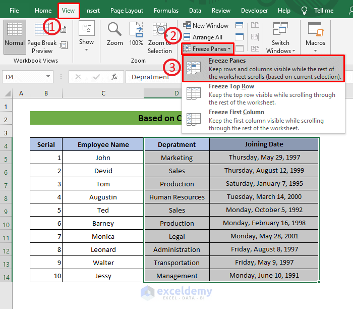
- Select Freeze Panes from the View tab.
- From the dropdown list, select Freeze Panes.
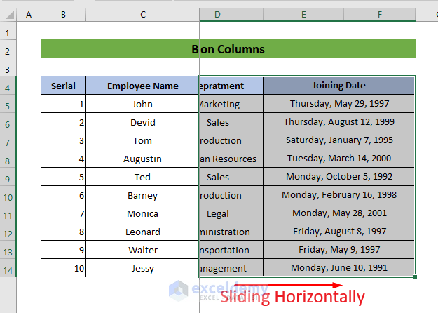
- You can now scroll horizontally with these two columns always visible.
Read More: How to Freeze Multiple Panes in Excel
Method 2 – Applying Excel Freeze Panes to Freeze Rows
Steps:
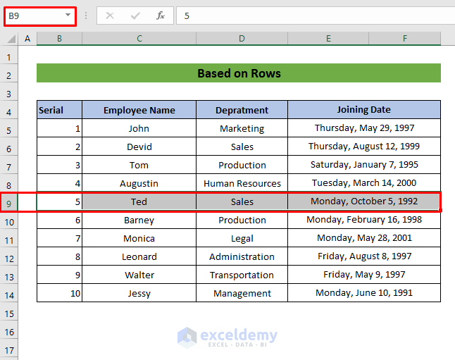
- We want to freeze the rows so the information for the first four employees shows, which ends at row 8. So, select row 9.
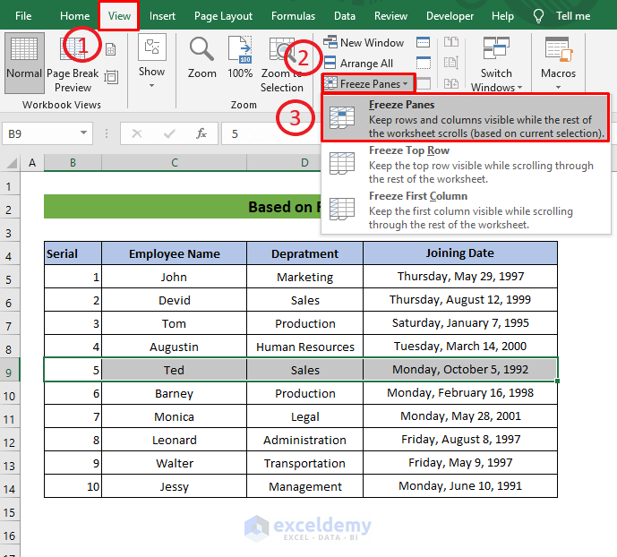
- Select Freeze Panes from the View tab.
- From the dropdown list, select Freeze Panes.
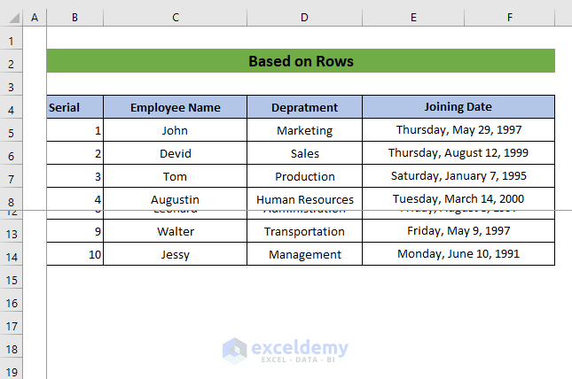
- You can now scroll down with these 4 rows always visible.
Method – Adding a Freeze Button to the Quick Access Toolbar to Freeze Columns and Rows at the Same Time
Steps:
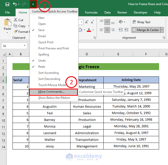
- Click the down arrow from the top of the Excel file.
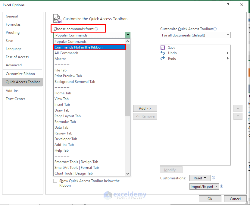
- Click More Commands from the drop-down list.
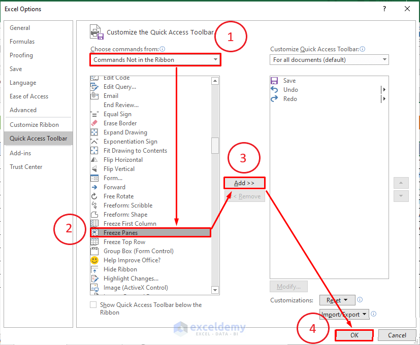
- Under Choose commands from, select Commands Not in the Ribbon.
- Select Freeze Panes and click Add.
- Click OK to add the command to the Quick Access Toolbar.
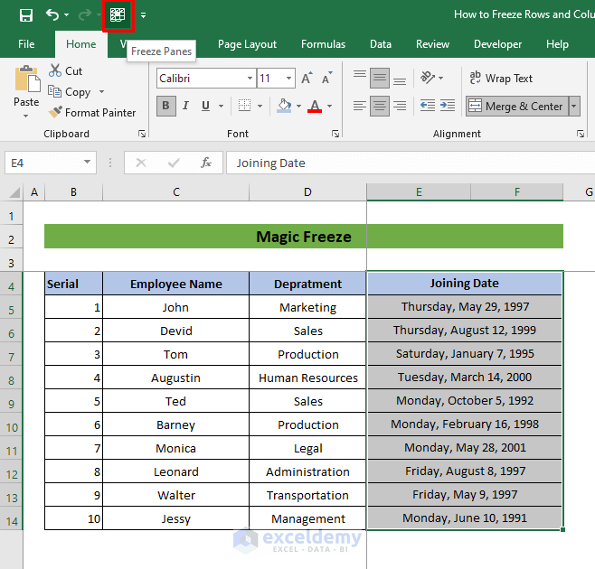
- To freeze rows and columns, select the first cell after the row and column you want to freeze.
- Click the Freeze Panes button and the columns and rows will be frozen at the same time.
Read More: How to Freeze Panes with VBA in Excel
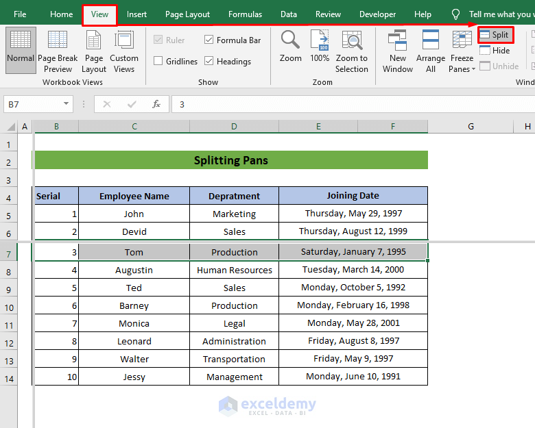
Method 4 – Splitting Panes to Freeze Rows and Columns Simultaneously
Steps:
- We want to freeze the first two rows (information of the first two employees) of the worksheet. So, we will select row 7.
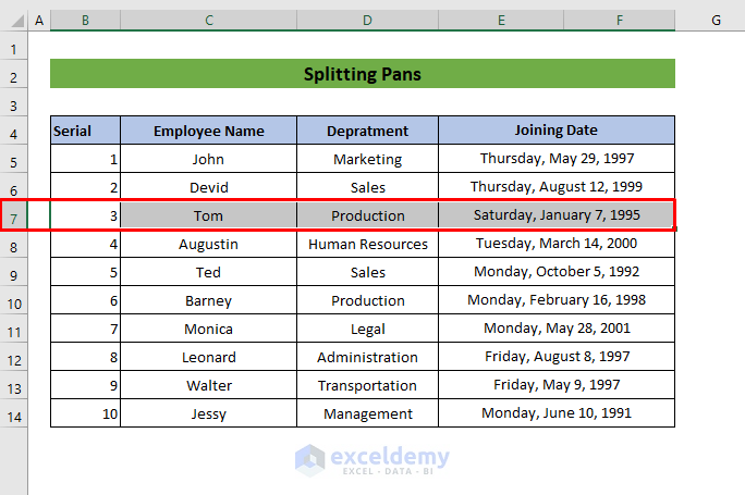
- On the View tab, click Split.
Things to Remember
- You can’t use Freeze Panes and Split Panes simultaneously.
- You have to select the row(s) below the one you want to be frozen or the column right of the column(s) you need to be frozen.
- If you want to freeze rows and columns at the same time based on a reference cell, the reference cell must be below the row and to the right of the column you want to freeze.
Download the Practice Workbook
Further Readings
- How to Freeze Top Row and First Column in Excel
- How to Unfreeze Rows and Columns in Excel
- Keyboard Shortcut to Freeze Panes in Excel
- How to Apply Custom Freeze Panes in Excel
- Excel Freeze Panes Not Working
<< Go Back to Freeze Panes | Learn Excel
Get FREE Advanced Excel Exercises with Solutions!

to freeze panes for both rows and columns at the same time i had to do method three but i had to click the row that i wanted it to stop at first (so row 4 in your example if I wanted the category to stay in place but the names to move) and the first cell of the column after the ones i wanted locked and below the row selected.(so if i wanted to freeze everything to the employee name i would select D5 so D and on would scroll)
Hello Rob,
Thanks for sharing your experience! You’re absolutely right—when freezing panes for both rows and columns, selecting the cell after the row and column you want to freeze is essential. In your case, selecting D5 allows the desired categories to remain visible while enabling the rest of the sheet to scroll. This method offers a great way to keep key information in view.
Regards
ExcelDemy
Sadly nothing i can do will restore my excel sheet to how it was originally. i had an excel sheet i was working in and i sudden;t found it was not possible to insert a new row. i kept getting a strange error message telling me that i have reached the limit of rows available, and i need to delete rows if i want to add a new row. This made no sense to me. I scrolled down to the bottom of my excel spreadsheet only to discover to my amazement that I had in excess of one million rows. I did not add these. I went through the typical process to delete rows, but no rows were being deleted. i wasted hours and hours and hours of my day trying in vain to delete 1 million, 48 thousand, 5 hundred and 75 rows… but not a single row was ever deleted. i then discovered something called ‘protected mode’ and found it was a ‘protected’ excel sheet, and i wanted to turn on deleting rows but strangely, it wants a password to do this!? This is my excel sheet, there is no password that i created to protect it, so i have no clue what happened there. So i selected all the rows i did want, and then created a new excel sheet from scratch, pasted all my rows and columns into it, re-arranged the column widths to how i want and THAT got rid of the more than 1 million redundant rows that excel mysteriously added. it is still in protected mode, and i don’t think i can ever remove this, but at least i got rid of all those million plus rows and can now add the rows i need and keep it limited to only the amount the sheet should have… but now, the rows and columns that i had before that were frozen so i could scroll right and down and keep the ones in place that i need to see, those are gone and won’t return. i can freeze the very top row, which is more or less a header and not really the first row, OR i can freeze the first column, but not both. i managed to do it on my previous excel sheet, but it had the 1,048,875 rows and i needed to limit it to 300 rows only which was impossible to do which is why i tried to copy and paste it into a new excel sheet in the first place, just to get rid of the redundant rows… so now what? nothing lets me freeze BOTH first column AND row 3. so HOW on earth did this happen, WHY is my excel sheet in a locked and protected mode with a password that i never set up and why did it add and never let me remove over a million rows that excel itself added without me knowing or wanting and WHY ON EARTH does excel refuse to let me freeze BOTH a column AND a row that i select!????? OMFG
Hello Au,
I’m sorry you’re facing such a frustrating issue. The huge number of rows appearing is likely due to unintended formatting or data extending to Excel’s maximum limit, causing the spreadsheet to appear full. Protected mode often activates automatically if the file was downloaded or from an external source. To freeze both rows and columns simultaneously, select the cell just below and to the right of the rows/columns you want frozen.
Example:
Select cell B4 if freezing column A and rows 1-3 then choose Freeze Panes again. Hope this helps!
Regards
ExcelDemy