You may have multiple columns in your spreadsheet while dealing with a large dataset. You need to freeze the columns at one place to scroll sidewise to the other columns to get the information properly. It is a very easy and handy process to freeze the columns. But when you need to return the dataset to its former state, you may find it difficult to unfreeze columns in Excel.
In this article, we are going to show you the simple and straightforward ways to unfreeze columns in Excel. We have demonstrated 3 useful methods here. If you go through the article, you can easily unfreeze your columns if they have been frozen. The below overview image depicts one of the methods to unfreeze columns using the Freeze Panes option.

How to Unfreeze Columns in Excel: 3 Quick Ways
It is important to unfreeze columns in Excel to get the proper information from your dataset. Otherwise, there may be a possibility that some data in a column hides in the frozen line. Whenever you work with a large dataset, it becomes important to freeze some rows and columns to scroll over all of the datasets. For showing you the way to unfreeze columns, we have taken a dataset of “IMDb Movies Database” where different movie-related info is stored.

There are no frozen columns in our above dataset. So, we have to apply any of the methods to freeze columns in Excel. Here, we have used the Freeze Panes option.
- First, you need to select the entire column just after the column you need to freeze.
- Then move to the View tab >> select Freeze Panes option from the Window group >> pick Freeze Panes.
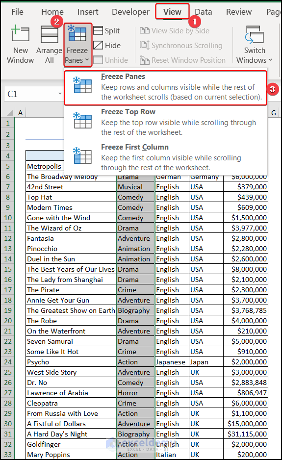
The grey line that appears indicates that column B is frozen. When you scroll the column sidewise the column will be hidden beneath the line.

Let’s come to the point. We want to unfreeze the frozen columns in Excel. To do this, follow the below 3 suitable methods.
1. Using Freeze Panes Option from View Tab
After freezing your columns, if you need to scroll all the information that is being stored under the grey line, you need to unfreeze the columns. Follow the below steps.
- Initially, you need to hover over the View tab >> choose Freeze Panes from the Window group >> pick Unfreeze Panes.

As you can see the grey line has disappeared which means you have done your job of unfreezing columns. See the below image for better clarification.

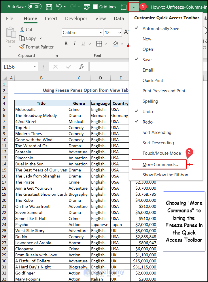
Note: You can bring the Freeze Panes option from the Quick Access Toolbar also. Follow the below process to do so.
- First, click on the Customize Quick Access Toolbar icon at top of your Excel sheet. Pick More Commands from there.
- The Excel Options window appears. From there, select the Freeze Panes and press Add>>.
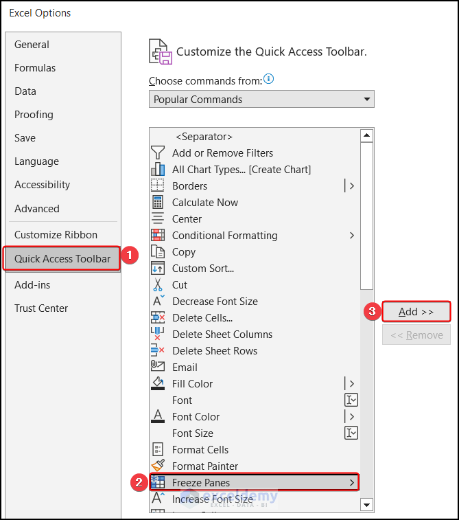
Finally, the Freeze Panes dropdown has been added at the top of your Excel workbook. You can Freeze/Unfreeze rows or columns from there.

Read More: How to Freeze Top Row in Excel
2. Applying Keyboard Shortcut to Unfreeze Columns
The keyboard shortcut also helps you to unfreeze columns in Excel. It is a fast and easy process, so it saves your valuable time. To use the keyboard shortcut,
- Firstly, press the ALT+W key on your keyboard. It will take you to the View tab.
- Eventually, a prompt will appear in the ribbon tab like the below image. Press the “F” key on your keyboard to open the Freeze Panes options from the Window group.

- Next, press the “F” key again to unfreeze the panes.

The below image indicates that there is no frozen line in the sheet.

So, the final keyboard shortcut is ALT + W + F + F. When you press the ALT + W + F + F keys together on your keyboard, you can unfreeze the columns in Excel.
Read More: How to Freeze Columns in Excel
3. Using VBA Macros to Unfreeze Columns in Excel
There is a simple VBA code that helps you to unfreeze columns automatically. It makes your dataset more dynamic when you use VBA. It automates and reduces the steps regarding this process. To use the VBA follow the below steps.
- First, go to the Developer tab >> choose Visual Basic.

Note: By default, the Developer tab remains hidden. In that case, you have to enable the Developer tab.
- The Visual Basic Editor window appears. Navigate the Insert tab >> select Module >> Module1.

- Write the following VBA code there.
Sub UnfreezeColumns()
ActiveWindow.FreezePanes = False
End Sub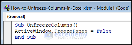
The code implies that if there are any freeze panes in the active window, then those will not be shown, as we entered the argument as False.
Finally, run the code with the F5 key, and the freeze line will disappear as in the image below.

Read More: How to Freeze 2 Columns in Excel
Frequently Asked Questions
- Can we freeze and unfreeze columns in the middle of a worksheet?
A: A worksheet’s center columns can indeed be frozen and unfrozen. To achieve this, click “Freeze Panes” and choose “Freeze Panes” from the dropdown menu, then choose the cell underneath and to the right of the rows and columns you wish to freeze. Click “Freeze Panes” once again and choose “Unfreeze Panes” to defrost.
- Can we unfreeze columns in Excel on a Mac?
A: Yes, by using the same procedures as on a Windows machine, you may unfreeze columns in Excel on a Mac. The “View” tab on the ribbon menu has the “Freeze Panes” button.
- Can we freeze and unfreeze rows and columns at the same time in Excel?
A: In Excel, you may freeze and unfreeze rows and columns simultaneously. Simply pick the cell underneath the final frozen row and to the right of the final frozen column, click “Freeze Panes,” and then choose “Freeze Panes” from the dropdown menu. Click “Freeze Panes” once again and choose “Unfreeze Panes” to defrost.
Things to Remember
- If the window has been divided into many panes, you can remove the frozen columns by moving the split bar to the right until they are no longer frozen.
- Simply scroll to the left until the columns you wish to unfreeze are visible if you’ve frozen the panes but want to keep the columns that are to the left of the frozen panes locked.
- If you are not sure enough about which columns need to be unfrozen then just use the “Unfreeze Panes” option to unfreeze columns.
Download Practice Workbook
Conclusion
We have come to the end of our article. With the help of this article, you can manipulate your data with ease. If the columns are frozen, you can easily unfreeze them using the methods described above. If you have any queries or any kind of Excel-related problems, you may contact us through emails or comments. Keep supporting us by providing your suggestions on where we can improve our quality.
Related Articles
- How to Freeze Top Two Rows in Excel
- How to Freeze Top 3 Rows in Excel
- How to Freeze First 3 Columns in Excel
- How to Freeze Random Selection in Excel
- How to Lock Cells in Excel When Scrolling
- How to Unlock Cells in Excel When Scrolling
- How to Lock Rows in Excel When Scrolling
<< Go Back to Unfreeze Panes | Freeze Panes | Learn Excel
Get FREE Advanced Excel Exercises with Solutions!
