How to Freeze Panes in Excel

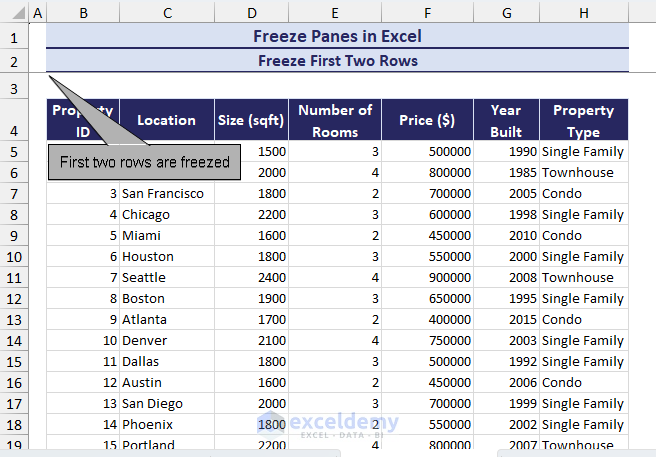
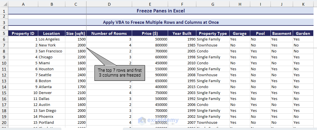
Consider the following dataset. It contains 60 rows and 11 columns. The top row is frozen.

Note

How to Freeze Rows in Excel

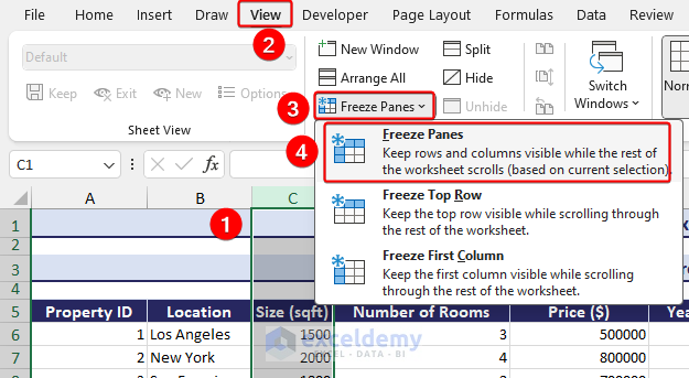
1. Freeze the Top Row

Click the View tab.
Select Freeze Panes.
Choose Freeze Top Row.

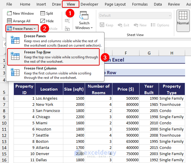
If you scroll down, the top row is visible.

Note

If you have frozen any other area of the worksheet, you must unfreeze it.

2. Freeze the Two Top Rows

Select the 3rd row.
Go to the View tab.
Select Freeze Panes.
Choose Freeze Panes.

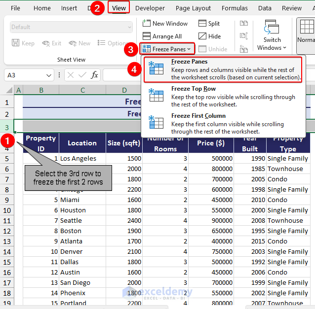
This is the output.

3. Freeze Multiple Rows

To freeze the first 13 rows:

Select the 14th row.
Go to the View tab.
Select Freeze Panes.
Select Freeze Panes.

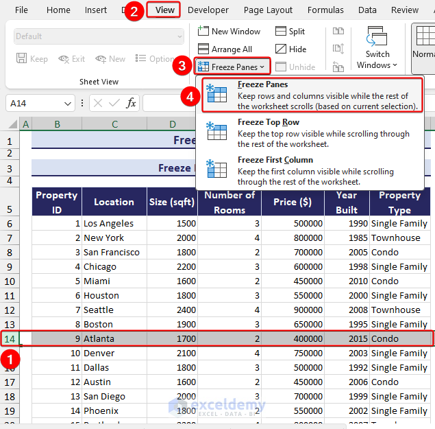
This is the output.

Note

You can’t freeze multiple rows or columns in different areas by using the Freeze Panes feature in Excel.

How to Freeze Columns in Excel

1. Freeze the Left Column

Go to the View tab.
Select Freeze Panes.
Select Freeze First Column.

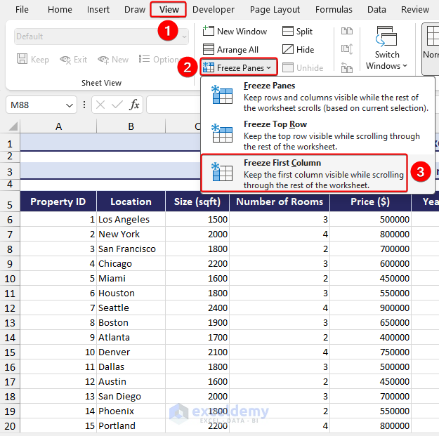
This is the output.

Note

You can’t freeze the top row and first column at a time.

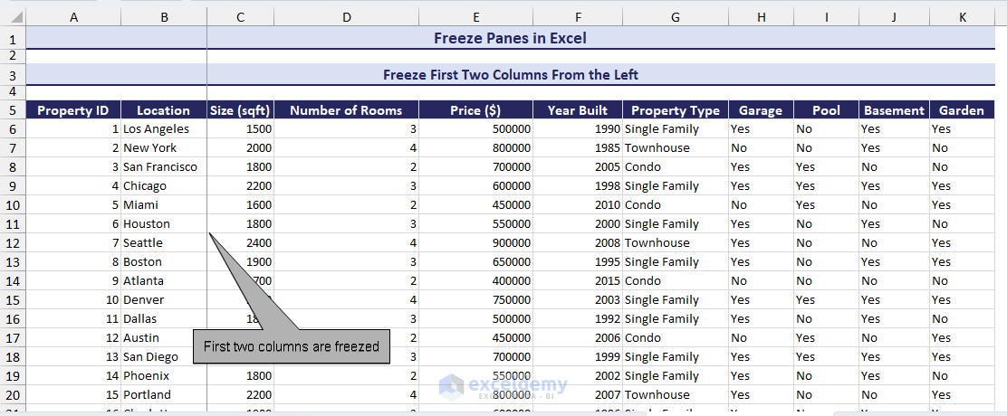
2. Freeze the First two Columns on the Left

Select column C.
Go to the View tab.
Select Freeze Panes.
Choose Freeze Panes.

This is the output.

first two column freezed using freeze panes feature

Click on the image for enlarged view

3. Freeze Multiple Columns

First, select the fourth column.
Go to the View tab.
Select Freeze Panes.
Choose Freeze Panes.

This is the output.

How to Freeze Multiple Rows and Columns in Excel

Select the cell that is located immediately below and to the right of the rows and columns you want to freeze. Here, D11.
Go to the View tab.
Select Freeze Panes.
Choose Freeze Panes.

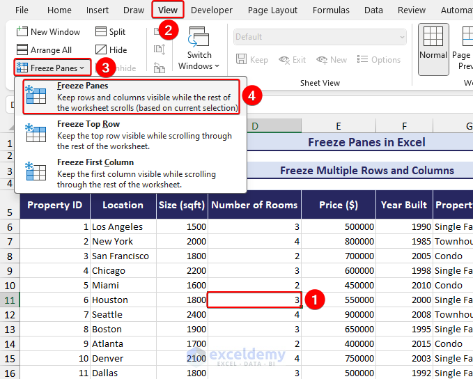
This is the output.

Note

If you enter the editing mode in a cell instead of selecting it, the Freeze Panes option will not be available.

Keyboard Shortcuts to Freeze Panes in Excel

Shortcuts	What It Does
Alt+W+F+R	Freeze Top Row
Alt+W+F+C	Freeze First Column
Alt+W+F+F	Freeze Top Row and First Column (Freeze Panes)
Alt+W+U	Unfreeze Panes

How to Apply VBA to Freeze Multiple Rows and Columns

Go to the Developer tab.
Select Visual Basic in Code.

Note

If you the Developer tab is not displayed on the Ribbon, enable it in Excel Options.

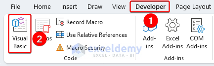
Click Insert and select Module.

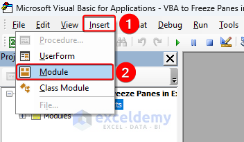
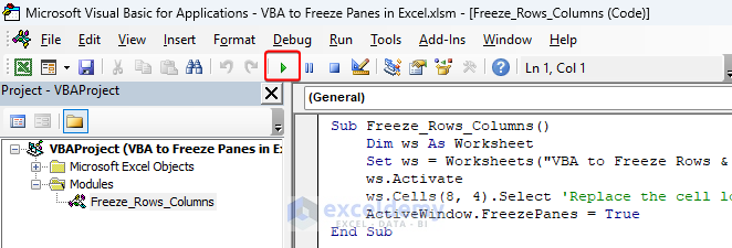
Copy this code into Module1.

Sub Freeze_Rows_Columns()
Dim ws As Worksheet
Set ws = Worksheets("Using_VBA") ' Replace with your sheet name
ws.Activate
ws.Cells(9, 5).Select 'Replace the cell location
ActiveWindow.FreezePanes = True
End Sub

Press F5 or click Run.

The first 7 rows and 3 columns are frozen.

Click on the image for enlarged view

Code Breakdown

Dim ws As Worksheet: Declares the “ws” variable of type “Worksheet”.
Set ws = Worksheets(“Using_VBA”): Assigns the worksheet “Using_VBA” to the “ws” variable.
Activate: Activates the worksheet referred to in the “ws” variable.
Cells(8, 4).Select: Selects the cell located in row 8 and column 5.
FreezePanes = True: Sets the “FreezePanes” property to “True“, which freezes the rows and columns above and to the left of the selected cell.

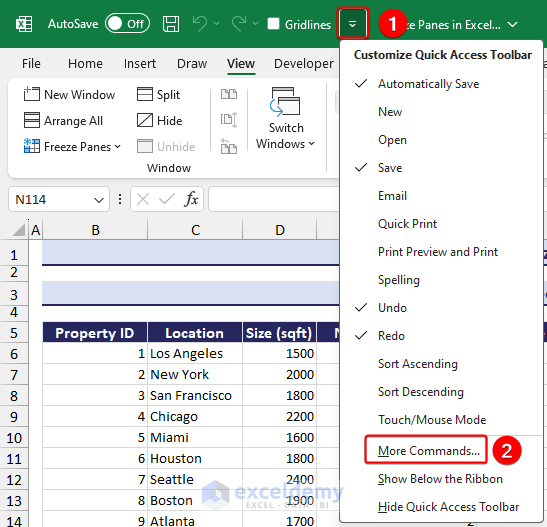
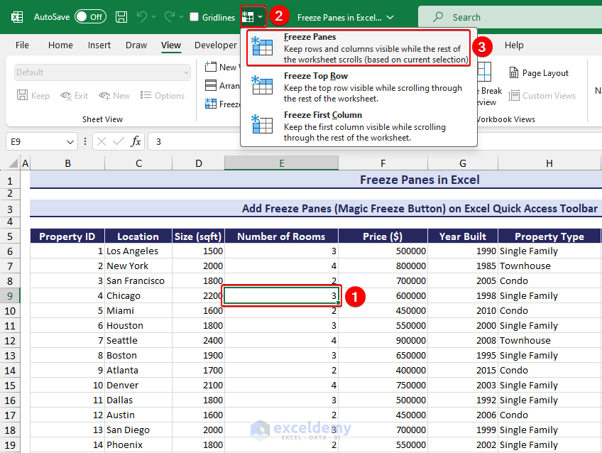
How to Add Freeze Panes (Magic Freeze Button) to the Excel Quick Access Toolbar

Click Customize Quick Access Toolbar (down arrow) at the top of the worksheet, and select More Commands.

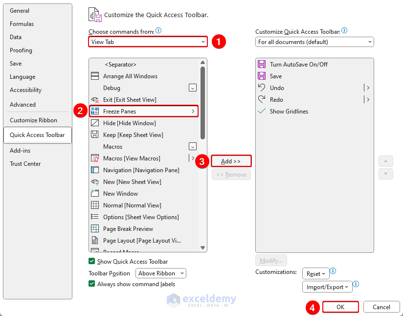
In Choose commands from, select View Tab.
Select Freeze Panes.
Click Add.
Click OK.

Adding the Freeze Panes option in the quick access toolbar in Excel

Click on the image for enlarged view

The Magic Freeze Button is displayed at the top of the toolbar.

Select a cell and click Freeze Panes.

freezing rows and columns using the quick access toolbar

Click on the image for enlarged view

This is the output.

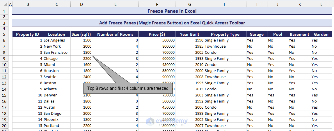
Click on the image for enlarged view

Navigating with Frozen Panes in Excel

Press Ctrl+Home to go to A1 when there are no frozen panes.

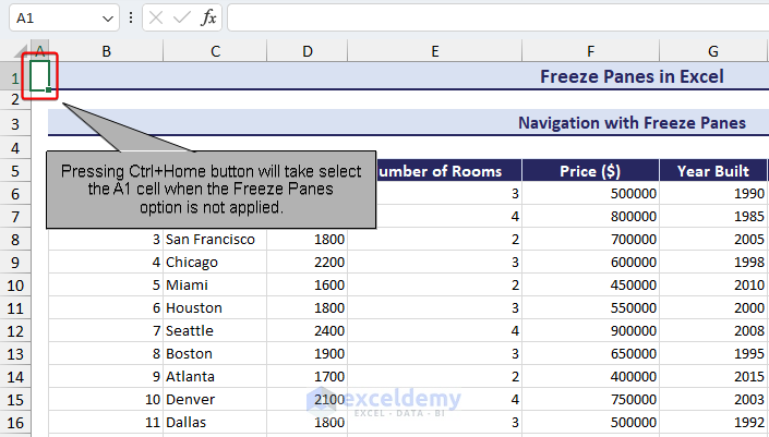
Freeze panes using the Freeze Panes feature.
Press Ctrl+Home to go to the first free cell in the worksheet.

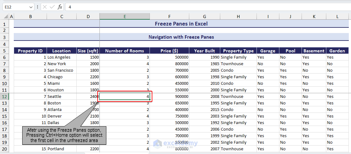
Navigation with Freeze Panes option applied

Click on the image for enlarged view

The first 11 rows and 4 columns are frozen. The first cell is E12.

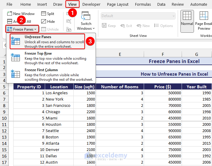
How to Unfreeze Panes in Excel

Go to the View tab.
Click Freeze Panes.
Select Unfreeze Panes.

Alternatives to Freezing Panes in Excel

1. Using the Split Option in the View Tab

Split Horizontally

Select an entire row.Here, row 12.
Click the View tab.
Select Split.

The worksheet is split horizontally.

Split Vertically

Click a column. Here, E.
Click the View tab.
Select Split.

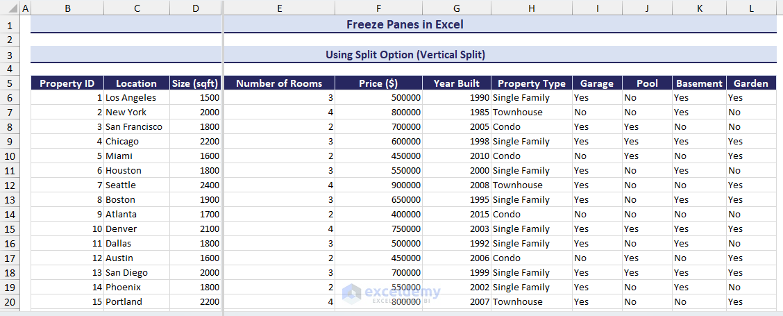
Click on the image for enlarged view

Split into Four Parts

Click a cell. Here, E14.
Select Split.

The worksheet is split into four parts. You can scroll each part individually.

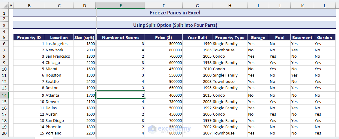
Click on the image for enlarged view

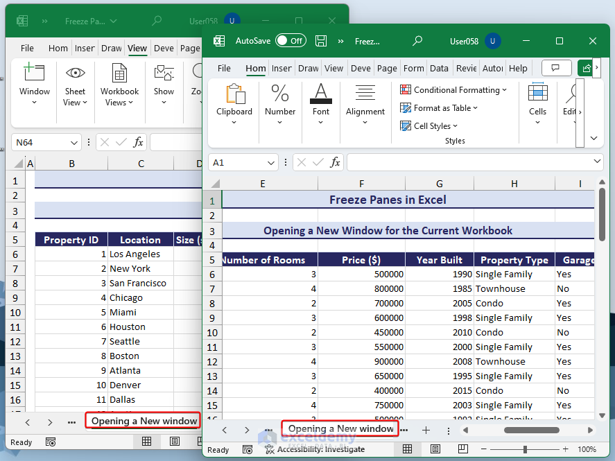
2. Opening a New Window in the Current Workbook

Click the View tab.
Choose New Window in Window.

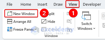
You can open the same sheet in different columns to compare data.

same sheet opened in a new window in stead of using freeze panes in Excel

Click on the image for enlarged view

3. Inserting a Table to Lock the First Row

Click a cell in the dataset.
Go to the Insert tab.
Choose Table.

Note

Alternatively, press Ctrl + T to insert a table.

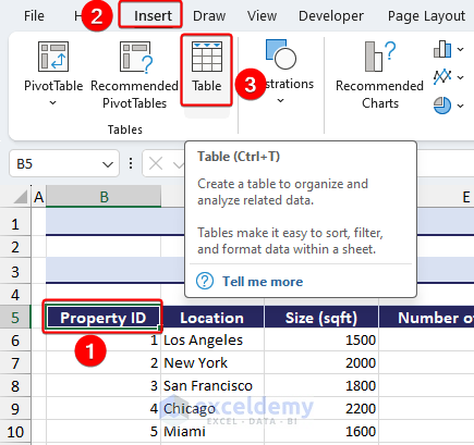
Select the Table.
Check My table has headers.

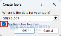
Click OK.

While scrolling, if you select any cell in the table, the table header row will always be visible.

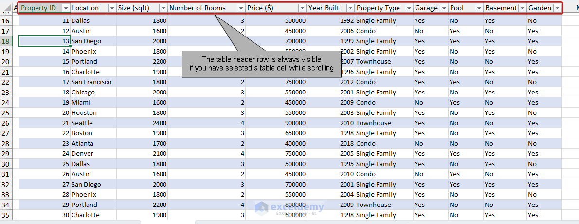
top row visible without using Excel Freeze panes feature

Click on the image for enlarged view

Reasons That Cause Freezing Panes Not to Work

You are in Page Layout view: change to Normal view.
You have already frozen rows or columns: unfreeze them before applying freeze panes to a different area.
The worksheet is protected.
You don’t have enough data to require a scroll bar.

Download Practice Workbook

Freeze Panes in Excel.xlsx

VBA to Freeze Panes.xlsm