This is an overview:
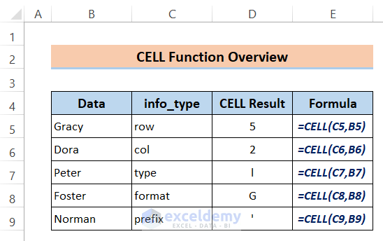
The CELL Function in Excel
Function Objective:
The CELL Function returns information about a cell color, filename, content, format, row, etc.
Syntax:
CELL(info_type, [reference])Arguments Explanation:
| ARGUMENTS | REQUIRED/OPTIONAL | EXPLANATION |
| type | Required | The type of information that you’d like to find in the cell. |
| range | Optional | The cell (or range) to get information from. If the range parameter is omitted, the CELL function will return information from the last cell that was changed. |
The Type Can be:
| VALUE | EXPLANATION |
| “address” | Subject (as text) of the reference cell. |
|
“col” |
the column number of the selected cell. |
|
“color” |
1 when the color is a minus value. Otherwise, 0. |
|
“contents” |
Values of the higher-left cell. |
|
“filename” |
The name of the file that holds the reference. |
|
“format” |
The number format of the specific cell. |
|
“parentheses” |
1 when the cell is formatted with parentheses. Otherwise, 0. |
|
“prefix” |
The label prefix of the specific cell. – When the cell is left-aligned, a single quote (‘). -When the cell is right-aligned, a double quote (“). -When the cell is center-aligned, a caret (^). – When the cell is fill-aligned, a backslash (\). -For all others, an empty text value. |
|
“protect” |
1 when the cell is locked. Otherwise, 0. |
|
“row” |
The row number of the specific cell. |
|
“type” |
“b” when the cell is vacant. “l” when the cell holds a text constant. For all others, “v”. |
|
“width” |
The rounded nearest integer which is the width of the column of the cell. |
CELL Format Codes:
| If the Format is | The cell function returns |
|---|---|
| General | “G” |
| 0 |
“F0” |
|
#,##0 |
“,0” |
|
0.00 |
“F2” |
|
#,##0.00 |
“,2” |
|
$#,##0_);($#,##0) |
“C0” |
|
$#,##0_);[Red]($#,##0) |
“C0-“ |
|
$#,##0.00_);($#,##0.00) |
“C2” |
|
$#,##0.00_);[Red]($#,##0.00) |
“C2-“ |
|
0% |
“P0” |
|
0.00% |
“P2” |
|
0.00E+00 |
“S2” |
|
# ?/? or # ??/?? |
“G” |
|
m/d/yy or m/d/yy h:mm or mm/dd/yy |
“D4” |
|
d-mmm-yy or dd-mmm-yy |
“D1” |
|
d-mmm or dd-mmm |
“D2” |
|
mmm-yy |
“D3” |
|
mm/dd |
“D5” |
|
h:mm AM/PM |
“D7” |
|
h:mm:ss AM/PM |
“D6” |
|
h:mm |
“D9” |
|
h:mm:ss |
“D8” |
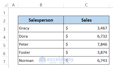
This is the sample dataset.
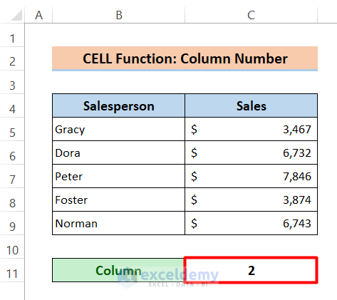
Example 1 – Return the Column Number with Excel CELL Function
Steps:
- Enter the following formula in C11:
=CELL("Col",B5)- Press Enter.
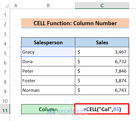
This is the output.
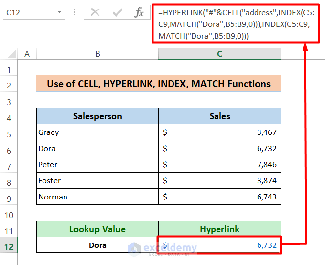
Example 2 – Combine the Excel CELL Function with the HYPERLINK, INDEX and MATCH Functions to Create a Hyperlink for a Lookup Value
Set the hyperlink for Dora.
Steps:
- Select C12.
- Enter the formula:
=HYPERLINK("#"&CELL("address",INDEX(C5:C9,MATCH("Dora",B5:B9,0))),INDEX(C5:C9,MATCH("Dora",B5:B9,0)))- Press Enter.
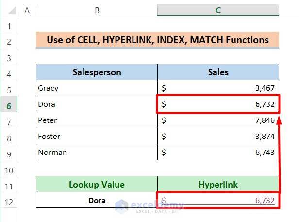
If you click the output, it will take you to the lookup result:
Formula Breakdown:
MATCH(“Dora”,B5:B9,0)
searches the ‘Dora’ in B5:B9 and returns its position in the selected array:
2
INDEX(C5:C9,MATCH(“Dora”,B5:B9,0))
returns the corresponding output according to that position in C5:C9:
6732
CELL(“address”,INDEX(C5:C9,MATCH(“Dora”,B5:B9,0)))
returns the cell address of 6732:
“$C$6”
HYPERLINK(“#”&CELL(“address”,INDEX(C5:C9,MATCH(“Dora”,B5:B9,0))),INDEX(C5:C9,MATCH(“Dora”,B5:B9,0)))
creates a link to the address $C$6 and returns:
6732
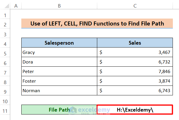
Example 3 – Combine the CELL Function with the LEFT and the FIND Functions to find the File Path
Steps:
- Enter the following formula in C11:
=LEFT(CELL("filename"),FIND("[",CELL("filename"))-1)- Press Enter.
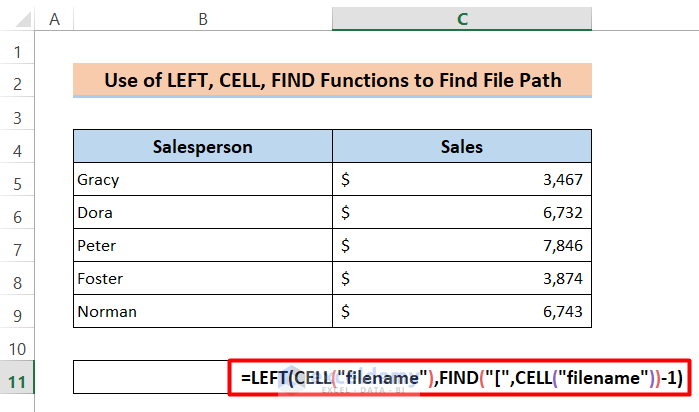
This is the file path:
 Formula Breakdown:
CELL(“filename”)
returns the full path, filename, and extension in square brackets, and sheet name:
“C:\Users\DELL\OneDrive\Desktop\mithun\45\[Excel_CELL_Function.xlsx]File Path”
FIND(“[“,CELL(“filename”))
returns the character position of “[” :
42
LEFT(CELL(“filename”),FIND(“[“,CELL(“filename”))-1)
returns 41 characters from the left to exclude “[”: 1 is subtracted from the previous output:
“C:\Users\DELL\OneDrive\Desktop\mithun\45\”
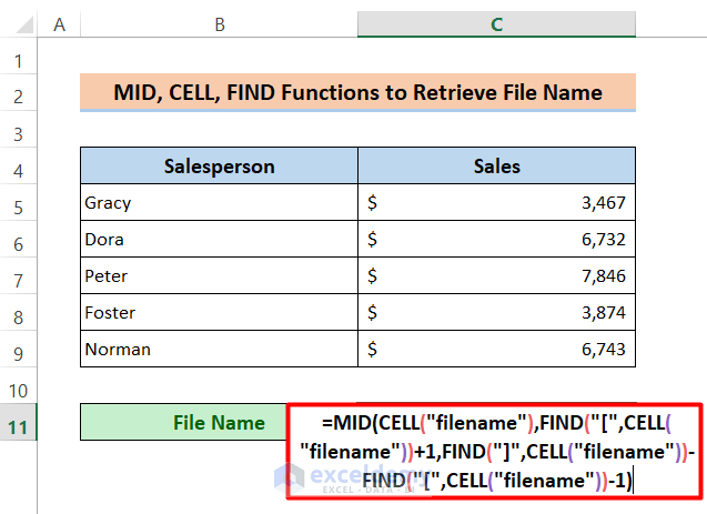
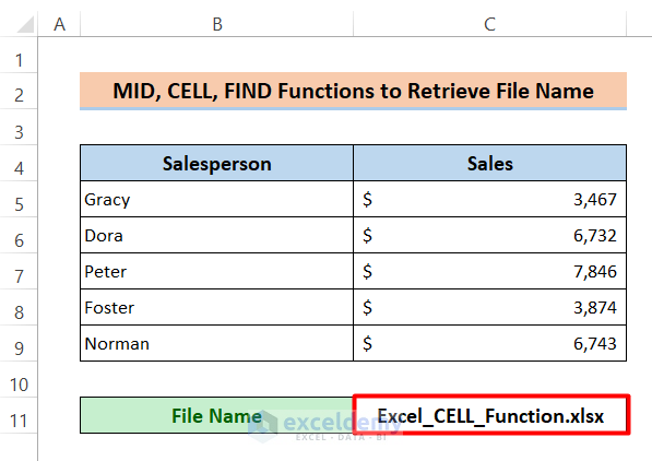
Example 4 – Use the CELL Function with the MID and the FIND Functions to get the Excel File Name
Steps:
- Enter the following formula in C11:
=MID(CELL("filename"),FIND("[",CELL("filename"))+1,FIND("]",CELL("filename"))-FIND("[",CELL("filename"))-1)- Press Enter.
This is the output.
Formula Breakdown:
CELL(“filename”)
returns the full path, filename, and extension in square brackets, and sheet name:
“C:\Users\DELL\OneDrive\Desktop\mithun\45\[Excel_CELL_Function.xlsx]File Name”
FIND(“[“,CELL(“filename”))
returns the character position of “[” :
42
FIND(“]”,CELL(“filename”))
returns the character position of “]” :
67
FIND(“]”,CELL(“filename”))-FIND(“[“,CELL(“filename”))-1
returns the sum:
24
FIND(“[“,CELL(“filename”))+1
returns the character position of “[” and adds 1:
43
➥ MID(CELL(“filename”),FIND(“[“,CELL(“filename”))+1,FIND(“]”,CELL(“filename”))-FIND(“[“,CELL(“filename”))-1)
keeps 24 characters starting from the position 43 and returns:
“Excel_CELL_Function.xlsx”
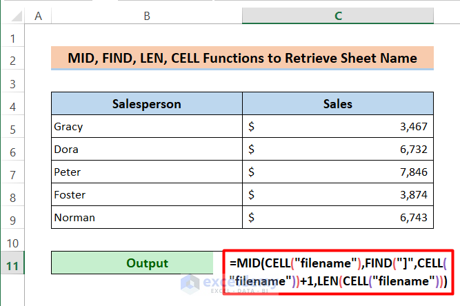
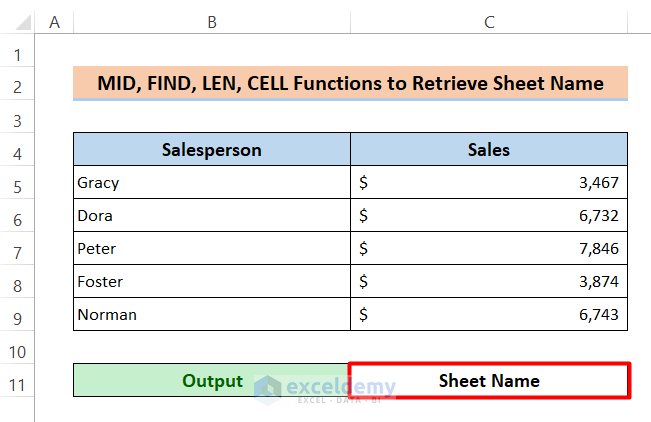
Example 5 – Combine the MID, FIND, LEN & CELL Functions to get the Sheet Name
Steps:
- Enter the following formula in C11:
=MID(CELL("filename"),FIND("]",CELL("filename"))+1,LEN(CELL("filename")))- Press Enter.
The sheet name is displayed.
Formula Breakdown:
CELL(“filename”)
returns the full path, filename, and extension in square brackets, and sheet name:
“C:\Users\DELL\OneDrive\Desktop\mithun\45\[Excel_CELL_Function.xlsx]Sheet Name”
LEN(CELL(“filename”))
counts the text length of the output of the CELL function:
77
FIND(“]”,CELL(“filename”))+1
finds the position of “]” and adds 1:
68
MID(CELL(“filename”),FIND(“]”,CELL(“filename”))+1,LEN(CELL(“filename”)))
returns the characters starting from the position 68:
“Sheet Name”
Download Practice Workbook
Download the free Excel template.
<< Go Back to Excel Functions | Learn Excel
Get FREE Advanced Excel Exercises with Solutions!

Can I apply this to filtered table?
Hello ROSEMARIE OLIVERA,
Thanks for your response. Yes, you can apply the CELL function to the filtered table.
Regards
MD Naimul Hasan