Download the Template
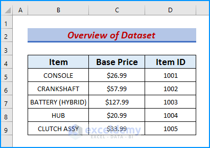
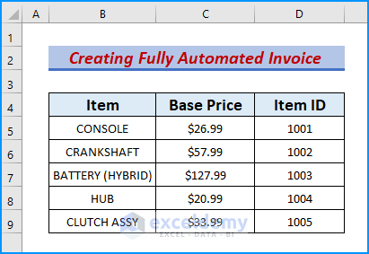
Excel functions such as the VLOOKUP, IFERROR, and SUM functions can be used to create fully automatic invoices. Use the Data Validation feature to implement the whole procedure. The dataset below represents auto parts item lists and prices of a company.
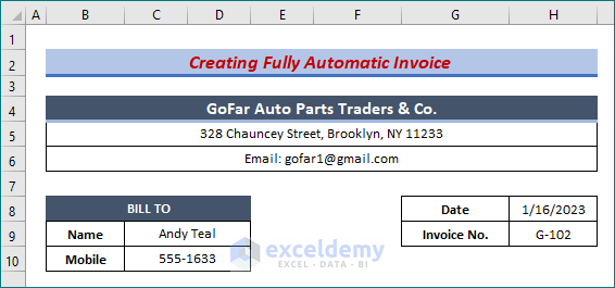
Step 1 – Basic Information of Fully Automatic Invoice
- In the merged cells, add the company name, company address, and email address.
- You can include Name, Mobile, Date & Invoice No. headers.
- Enter the correct values under each header.
- In the headers, add Item, Base Price, and Item ID (in B4, C4, and D4 respectively).
- Input correct information in each column.
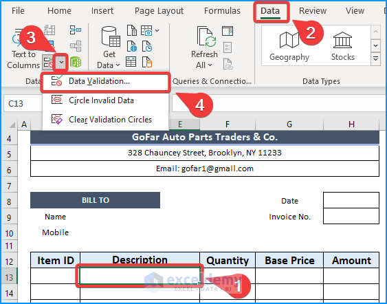
Step 2 – Utilize the Data Validation Feature to Import Data from Table Array
- Select cell C13.
- Go to the Data tab.
- Select Data Validation then go to Data Validation.
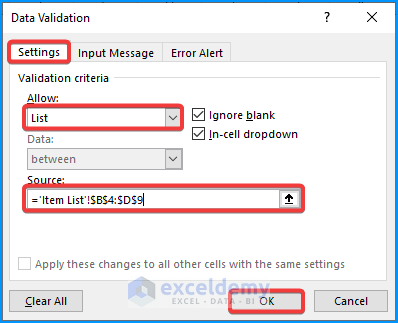
- The Data Validation will dialog box pop up.
- Select Settings.
- Choose List in the Allow box.
- In the Source box, select the table of Step 1.
- Click OK.
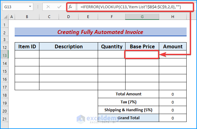
Step 3 – Combine VLOOKUP and IFERROR Functions to Display Data
- Enter the following formula in G13:
=IFERROR(VLOOKUP(C13,'Item List'!$B$4:$C$9,2,0),"")- Press the Enter or Tab button.
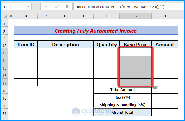
- Use the AutoFill tool to fill the formula to the rest of the cells in column G.
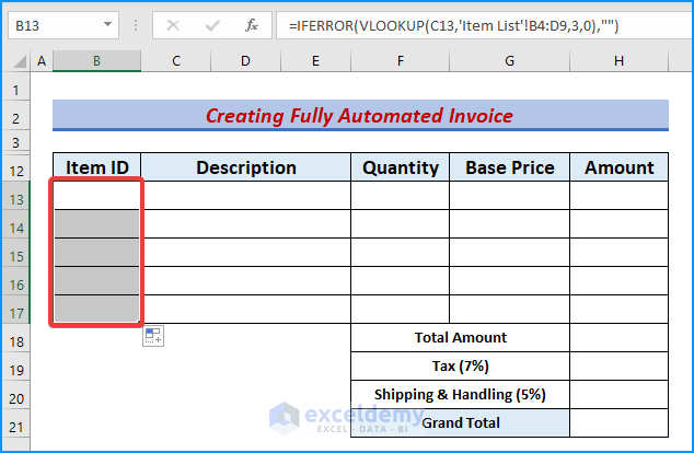
- Enter the following formula in B13:
=IFERROR(VLOOKUP(C13,'Item List'!$B$4:$D$9,3,0),"")- Press Enter.
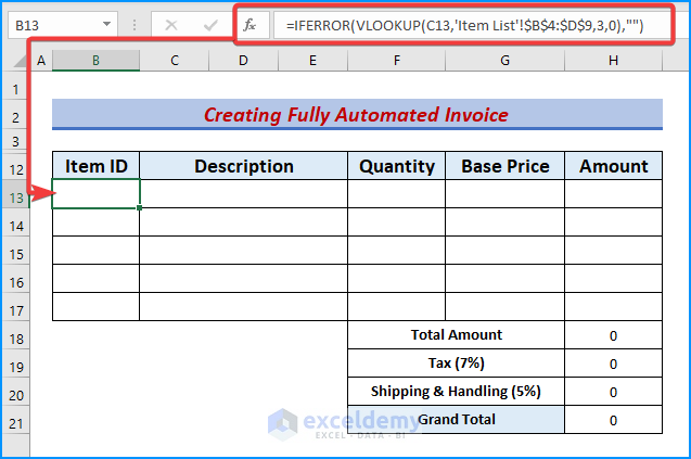
- Drag the formula cell down to AutoFill the whole column.
Formula Breakdown:
- VLOOKUP(C13,’Item List’!$B$4:$C$9,2,0) looks for the corresponding 2nd row of the data in C13 from the range B4:C9 of the Item List table.
- IFERROR(VLOOKUP(C13,’Item List’!$B$4:$C$9,2,0),””) returns a blank cell if it finds any missing or error data.
Read More: How to Create Proforma Invoice in Excel (Download Free Template)
Similar Readings
- Transport Bill Format in Excel (Create in 4 Simple Steps)
- How to Create a Cash Bill Format in Excel (A step-by-step Guideline)
- Create GST Invoice Format in Excel (Step-by-Step Guideline)
Step 4 – Join SUM and IFERROR Functions to Calculate Invoice Data
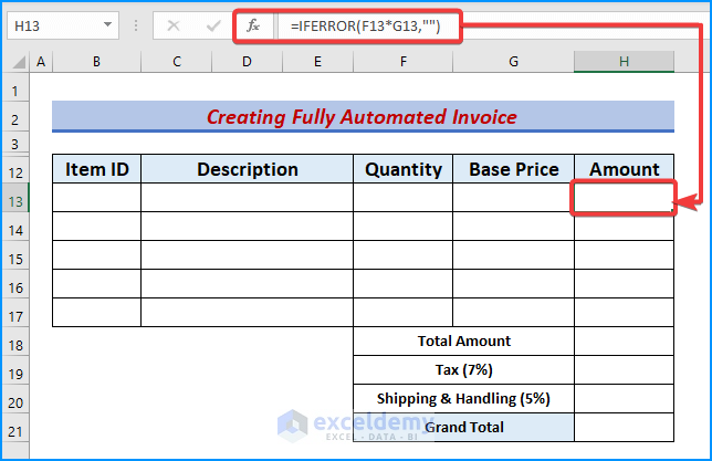
- Enter the following combined formula in H13:
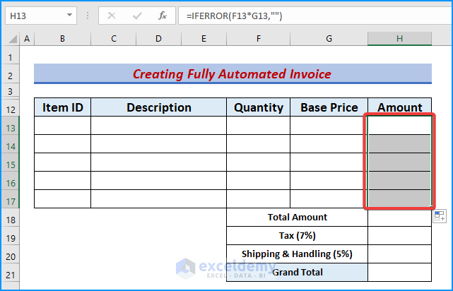
=IFERROR(F13*G13,"")- Press Enter.
- Use the AutoFill icon to drag the formula cell down.
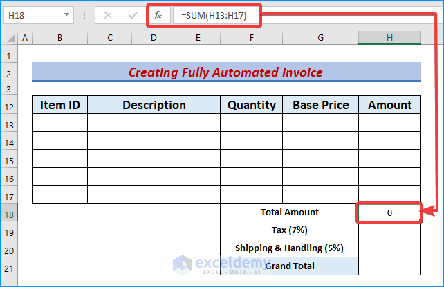
- In the cell H18, enter the following formula:
=SUM(H13:H17)- Press Enter.
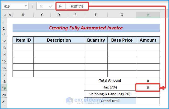
- Calculate the Tax with the formula below:
=H18*7%- Press Enter.
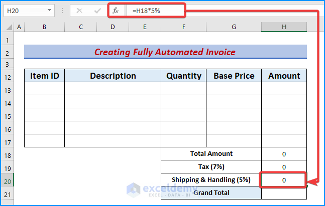
- To count the Shipping & Handling charges, enter the formula in H19:
=H18*5%- Press Enter.
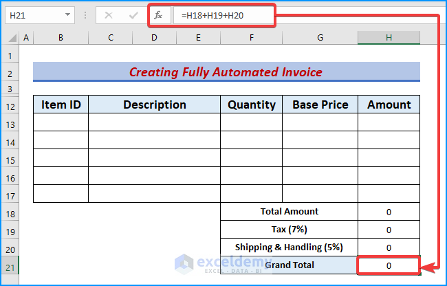
- To calculate the Grand Total, enter the given formula in H21:
=H18+H19+H20- Press Enter.
Read More: Tax Invoice Format in Excel (Download the Free Template)
Step 5 – Input Data and Analyze the Invoice Model
- Click any cell under the Description column and look for a dropdown icon.
- Tapping the Dropdown icons will display the item list.
- Select any item and type the number of items in the Quantity column.
- The desired Grand Total will show in our dataset.
Related Articles
- Use Electricity Bill Calculation Formula in Excel
- Create Invoice in Word from Excel Data (with Easy Steps)
- Labour Contractor Bill Format in Excel (Download Free Template)
- Hotel Bill Format in Excel (Create with Easy Steps)
- Excel Invoice Tracker (Format and Usage)

