Type 1 – Making a Bill of Materials for a Single Product
Step 1. Create a Basic Dataset for Making a Bill of Materials
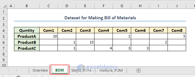
We have taken a dataset where there are some product lists with the components needed to make the product. We‘ll utilize these data to make a BOM.
Step 2. Prepare a Helping Table
We must make the helper columns to create the BOM for a single product.
- Enter the following formula into cells with the Fill Handle:
=OFFSET(BOM!$C$4,,ROW()-8,,)In our dataset, the Component Quantity is the total number of components used for a selected product, whereas the Component with Quantity measures the number of individual components of the product.
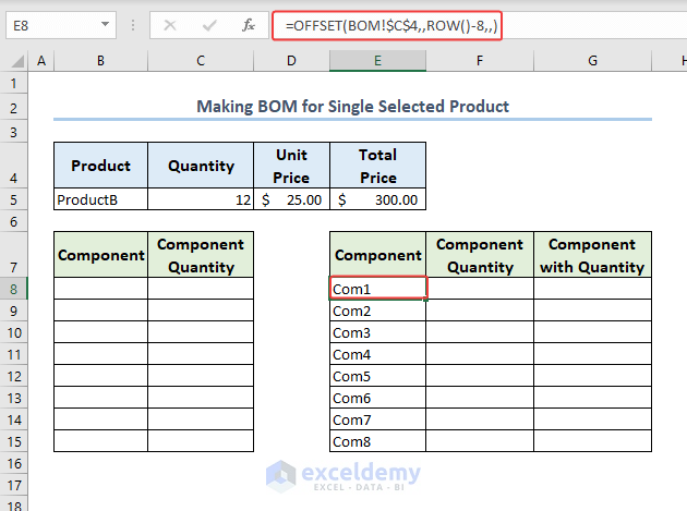
In the code, the OFFSET function in Excel is used to reference a range of cells based on a starting point and specified rows and columns. This formula references the range starting from cell BOM!$C$4 and adjusts the row offset based on the current row minus 8. The range referenced will have the same number of rows as the current row and extend horizontally from the starting cell.
- Enter the following formula in Cell F8 to find the required components for a product.
- Use the Fill Handle to copy the formula in the following cells.
=IFERROR(INDEX(BOM!$C$4:$ZZ$9999,MATCH($B$5,BOM!$B$4:$B$9999,0),MATCH(E8,BOM!$C$4:$J$4,0)),0)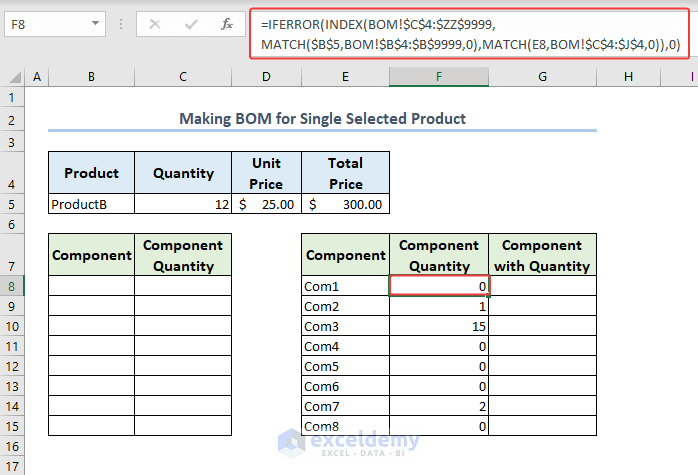
Formula Breakdown
- INDEX(BOM!$C$4:$ZZ$9999, MATCH($B$5, BOM!$B$4:$B$9999, 0), MATCH(E8, BOM!$C$4:$J$4, 0))
The INDEX function retrieves the value from a range (BOM!$C$4:$ZZ$9999) based on the row and column numbers provided by the MATCH functions.
The first MATCH function (MATCH($B$5, BOM!$B$4:$B$9999, 0)) searches for the value in cell $B$5 in the range BOM!$B$4:$B$9999 and returns the row number where a match is found.
The second MATCH function (MATCH(E8, BOM!$C$4:$J$4, 0)) searches for the value in cell E8 in the range BOM!$C$4:$J$4 and returns the column number where a match is found.
- IFERROR(formula, 0)
The IFERROR function checks if the formula in step 1 returns an error.
If there is an error (e.g., no match found), it returns 0. Otherwise, it returns the value from the BOM sheet.
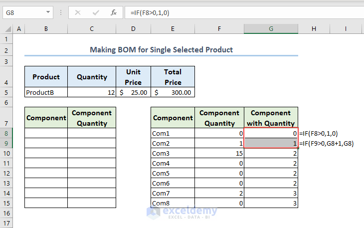
- Afterward, count the number of components for a product. Use the given formulas.
In cell G8.
=IF(F8>0,1,0)In cell G9.
=IF(F9>0,G8+1,G8)- Copy the second formula in the following cells using the Fill Handle.
Step 3. Find Component and Component Quantity for Single Selected Item
- Enter the following formula in cell B8 to get the required components for a selected product from the list.
- Use Fill Handle to copy the formula.
=IFERROR(INDEX(E:E,MATCH(ROW()-7,G:G,0),1),"")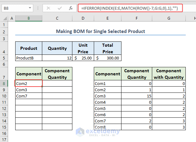
Formula Breakdown:
- INDEX(E:E, MATCH(ROW()-7, G:G, 0), 1)
The INDEX function retrieves the value from column E based on the row number provided by the MATCH function.
The MATCH function (MATCH(ROW()-7, G:G, 0)) searches for the row number (offset by 7) in column G and returns the position of the matched row.
- IFERROR(formula, “”)
The IFERROR function checks if the formula in step 1 returns an error.
If there is an error (e.g., no match found), it returns an empty string (“”). Otherwise, it returns the value from column E.
- Next, find the Component Quantity by using the following formula. Copy the formula in the following cells with the Fill Handle.
=IFERROR($C$5*INDEX(F:F,MATCH(ROW()-7,G:G,0),1),"")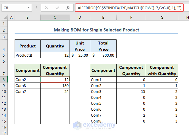
Formula Breakdown:
- $C$5 * INDEX(F:F, MATCH(ROW()-7, G:G, 0), 1)
The INDEX function retrieves the value from column F based on the row number provided by the MATCH function.
The MATCH function (MATCH(ROW()-7, G:G, 0)) searches for the row number (offset by 7) in column G and returns the position of the matched row.
The retrieved value from column F is then multiplied by the value in cell $C$5.
- IFERROR(formula, “”)
The IFERROR function checks if the formula in step 1 returns an error.
If there is an error (e.g., no match found), it returns an empty string (“”). Otherwise, it returns the result of the multiplication.
Step 4. Calculate the Total Price of the Product
- Enter the following formula to calculate the total price of the product. We assumed the unit price was $25.
=C5*D5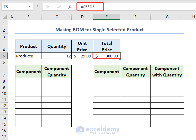
Type 2: Making a Bill of Materials for Multiple Products
Step 1. Modify for Finding Component and Component Quantity for Multiple Selected Products (Helper Table)
- Enter the following formula in Cell B6 to enlist the component quantity for each component for multiple selected products.
- Copy the formula in the following cells with the Fill Handle.
=IFERROR($C16*INDEX(BOM!$C$4:$ZZ$9999,MATCH($B16,BOM!$B$4:$B$9999,0),MATCH(B$4,BOM!$C$4:$J$4,0)),0)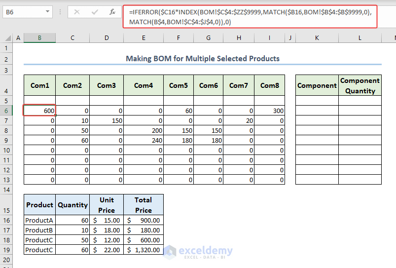
Formula Breakdown:
- $C16 * INDEX(BOM!$C$4:$ZZ$9999, MATCH($B16, BOM!$B$4:$B$9999, 0), MATCH(B$4, BOM!$C$4:$J$4, 0))
The INDEX function retrieves the value from the BOM range (BOM!$C$4:$ZZ$9999) based on the row and column numbers provided by the MATCH functions.
The first MATCH function (MATCH($B16, BOM!$B$4:$B$9999, 0)) searches for the value in cell $B16 in the range BOM!$B$4:$B$9999 and returns the row number where a match is found.
The second MATCH function (MATCH(B$4, BOM!$C$4:$J$4, 0)) searches for the value in cell B$4 in the range BOM!$C$4:$J$4 and returns the column number where a match is found.
The retrieved value from the BOM range is then multiplied by the value in cell $C16.
- IFERROR(formula, 0)
The IFERROR function checks if the formula in step 1 returns an error.
If there is an error (e.g., no match found), it returns 0. Otherwise, it returns the result of the multiplication.
- Calculate the total requirement of a component for all selected products.
- Enter the following formula in Cell B5:
=SUM(B6:B13)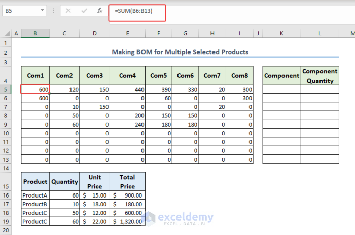
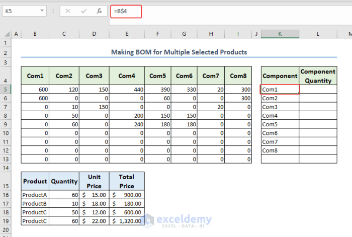
Step 2. Determining Component Name and Component Quantity
- Enter the component names in cell range K5:K12.
- Enter the following formula in cell L5 to get the component quantity required.
- Copy the formula in the following cells with the Fill Handle.
=HLOOKUP(K5,$4:$5,2,0)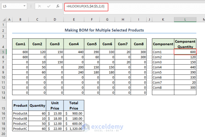
- In the formula, The HLOOKUP function searches for the value in cell K5 within the range of rows 4 to 5 ($4:$5). It returns the value from the second row of the matched column. The final argument of 0 specifies an exact match.
Step 3. Determine the Total Price of the Product
- Enter the following formula to get the total price of products:
=C16*D16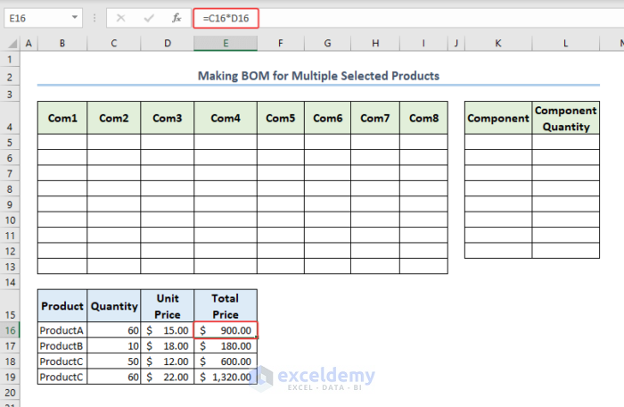
In the formula, we multiplied the Unit Price by Quantity to get the Total Price.
Things to Remember
- Be careful regarding the Cell reference used in the formulas.
- Use the Fill Handle to avoid the repetition of writing the same formula.
Download Practice Workbook
You can download the practice workbook from here.
Get FREE Advanced Excel Exercises with Solutions!
