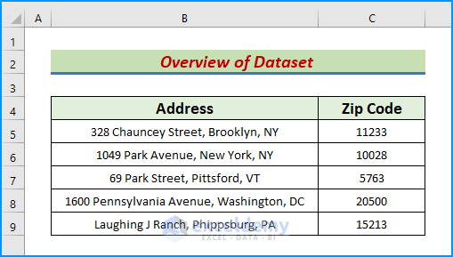
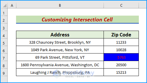
An intersection occurs when two or more lines or areas cross one another. The resulting shared point or area is known as the intersection point or area. Let’s take a dataset that represents U.S. addresses and their zip codes for demonstration. We’ll show the cell or range that is the intersection of two ranges.
Example 1 – Display the Intersection Point Address Utilizing the VBA Intersect Method in Excel
Step 1:
- Go to the Developer tab and click Visual Basic.
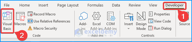
- The Visual Basic window pops up.
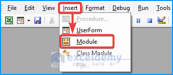
- Go to Insert and then select Module to create a module box.
Step 2:
- Insert the following VBA Intersection code in the module box. Include 2 ranges from the dataset.
Sub Dis_Inter_Address()
Dim MyOutput As Variant
MyOutput = Intersect(Range("C5:C9"),
Range("B7:C7")).Address
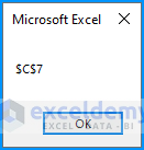
MsgBox MyOutput
End Sub
- Press the F5 key or the green Run icon.
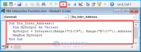
- Thus, we obtain the desired intersection cell address in a message box.
Code Breakdown:
- Dim MyOutput As Variant: Here, we declare a Variant namely MyOutput instead of a Variable.
- MyOutput = Intersect(Range(“C5:C9”), Range(“B7:C7”)).Address: Now, in the Intersect formula, we put 2 ranges (C5:C9) and (B7:C7) in the declared Variant and add the Address object to get the intersect cell address.
- MsgBox MyOutput: Finally, the MsgBox application displays the intersect point address.
Example 2 – Highlight the Intersection Cell Using the VBA Application.Intersect Formula in Excel
Steps:
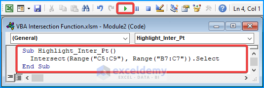
- Create a Module box.
- Input the following VBA Intersect formula.
Sub Highlight_Inter_Pt()
  Intersect(Range("C5:C9"), Range("B7:C7")).Select
End Sub
- The Intersect function determines the intersection point between the 2 ranges. Further, the Select application returns a selection in the dataset.
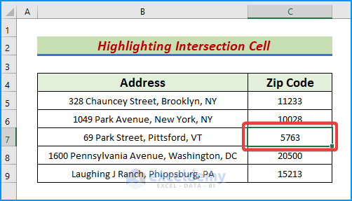
- After pressing the green Run icon, close the window tab.
- We get the intersection cell of the ranges selected.
Example 3 – Remove the Intersection Cell in Excel
Steps:
- Create a Module box and insert the following VBA code.
Sub Rem_Inter_Point()
  Intersect(Range("C5:C9"), Range("B7:C7")).ClearContents
End Sub
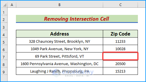
- Press the F5 key or the Run icon and close the tab.

- We removed the data of the intersection cell C7.
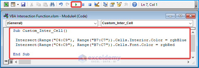
Example 4 – Customize Cell Colors and Font Colors at the Intersection Cell
Steps:
- Use the following code in the module:
Sub Custom_Inter_Cell()
 Intersect(Range("C4:C9"), Range("B7:C7")).Cells.Interior.Color = rgbBlue
 Intersect(Range("C4:C9"), Range("B7:C7")).Cells.Font.Color = rgbRed
End Sub
- Press the Run icon. The Intersect() function returns the intersection point of the given ranges.
- The Color and Font.Color applications change the obtained cell’s interior and font color respectively.
- We changed the interior cell color and font color of the intersection cell.
Notes:
- To ensure that the code runs every time, save the file in the Excel Macro Enabled Workbook format.
Download the Practice Workbook
Get FREE Advanced Excel Exercises with Solutions!

