The HYPERLINK function belongs to the Excel Lookup and Reference functions category. The function aids in the linking of data across several documents. This article explains almost everything about the HYPERLINK function in Excel.
HYPERLINK Function: Syntax and Arguments
The HYPERLINK function brings out a cutoff link that will open on a server, or make a move to other worksheets. Excel opens the URL when we click the cell that holds the HYPERLINK function.
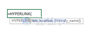
➧Syntax
HYPERLINK(link_location, [friendly_name])
➧Arguments
| Argument | Required/Optional | Explanation |
|---|---|---|
| link _location | Required | This is the path to the file or page or document that needs to be opened. |
| friendly_name | Optional | This is the text string or numerical value that is displayed as a link in the cell. |
➧Return Value
A clickable hyperlink.
How to Use Excel HYPERLINK Function: 8 Examples
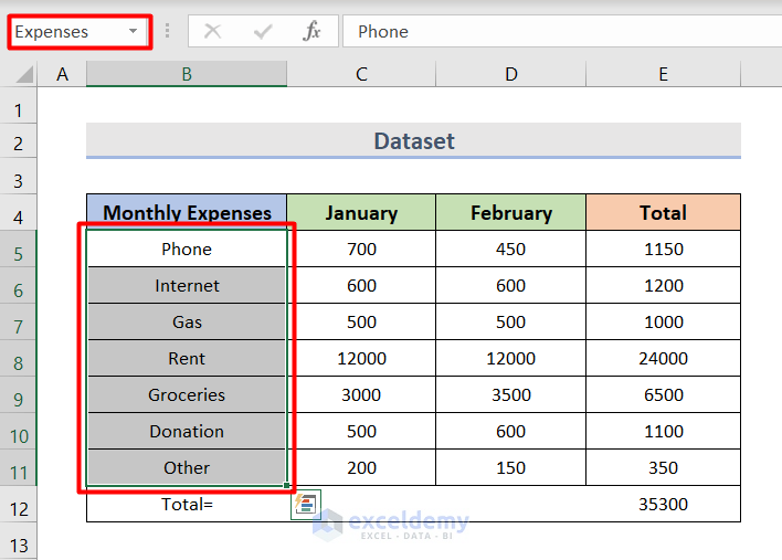
For using the HYPERLINK Function, we have used the following example. The following dataset which is in Sheet2 contains the monthly expenses and the total expenses for 2 months.
1. HYPERLINK to Different Worksheet in the Same Workbook
To insert the HYPERLINK function to another worksheet in the same workbook, write the pound sign (#) before the target sheet name inside a double quotation(“”). In cell C5 we will use the below formula to jump another worksheet.
=HYPERLINK(“#Sheet2!A1”, “Sheet2”)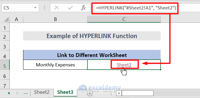
2. HYPERLINK to Different Workbook
We need to establish the full path to the target workbook to insert the HYPERLINK function. We can write the location in a cell and the friendly name in another cell to simply insert the HYPERLINK or,
=HYPERLINK(“D:\Source data\Book3.xlsx”, “HYPERLINK Function”)Instead of this, We can also keep the location in one cell and the friendly name in another cell. For example, we keep our location in cell B6 and the friendly name is in cell C6. Now, the formula for the HYPERLINK in cell D6 is:
=HYPERLINK(B6,C6)This will take us to another workbook where we want to work.
3. HYPERLINK to a Named Range
We can also link to named ranges. Named ranges just highlight the cells we want to name. In the following example, we named the range (B5:B11) expenses, which are located in Sheet2. Let’s pull the Named Range, add the pound (#) sign before it, and wrap it in quotation marks. Now, the formula will look like this:
=HYPERLINK(“#Expenses”, “List of Expenses”)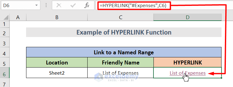
So this will create a link with that specific named range. If you click on that link, this will take you to the location of that named range.
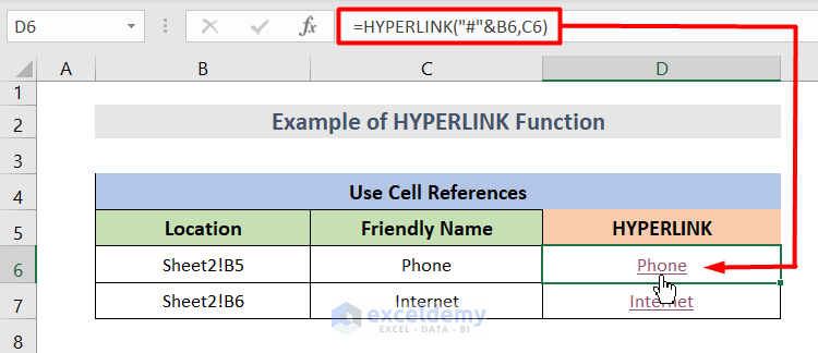
4. HYPERLINK to Cell Reference
The HYPERLINK function can move the cell reference to the same workbook in different sheets. For this, we have to put a pound sign (#) enclosed with a double quotation and then a ‘&’ before the sheet name. So, the formula will be:
=HYPERLINK(“#”&Sheet2!B5, “Phone”)Alternatively, we can directly link to the cell reference by keeping the location and friendly name in different cells, just shown in the picture below.
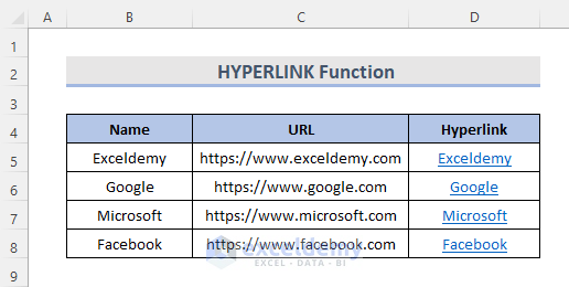
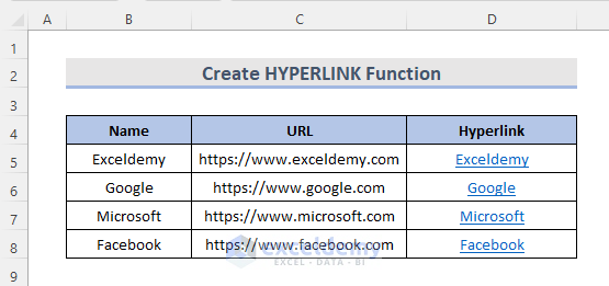
5. Create HYPERLINK to a Web Page
When we enter a URL in Excel, it automatically converts into a hyperlink. And when we click it, it takes us to the website. However, the HYPERLINK function will allow us to add a friendly_name.
So here is the address of our website, Exceldemy.com in cell C5. Using the HYPERLINK function the formula will look like this.
=HYPERLINK(“https://www.exceldemy.com”, “Exceldemy”)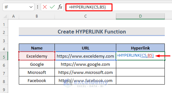
Then, if we want more hyperlink addresses using the function, simply drag the (+) sign below on the Excel sheet.
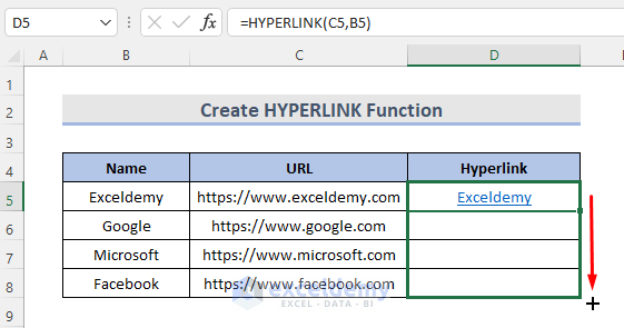
This will create the hyperlinks with a friendly_name. If we click on any of the hyperlinks, this will take us to the websites.
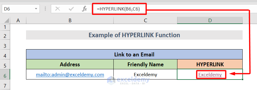
6. Excel HYPERLINK Function to Send an Email
The HYPERLINK function can create a new message for a specific recipient. To use the HYPERLINK function, we need to add mailto: at the start of the address.
=HYPERLINK(“mailto:[email protected]”, “Exceldemy”)Rather than writing the whole formula, we can just keep the address and the friendly name in other cells and the link in different cells.
Suppose, we put the address in cell B6 and the friendly name in cell C6. And we want to link to an email in cell D6. Now, the formula will be shorter like this:
=HYPERLINK(B6,C6)This adds a hyperlink to the workbook, and clicking the link creates a new message for our support team.
7. INDEX and MATCH Functions Wrapped with HYPERLINK Function
To generate hyperlinks that fetch a matching value and create a shortcut to it, utilize the HYPERLINK function with the INDEX and MATCH functions.
If we are working with a lot of data, It can be more useful to have the hyperlink point to the first cell in the row where the match is found. Simply set the return range in the first INDEX and MATCH combination to columns to do this.
=HYPERLINK("#"&CELL("address", INDEX(B5:B9, MATCH(E5, C5:C9,0))), INDEX(B5:B9, MATCH(E5, C5:C9,0)))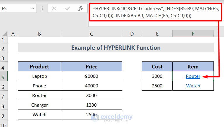
🔎 How Does the Formula Work?
- The Excel INDEX function returns a value in an array based on the row and column numbers.
- To find the first occurrence of the lookup value in the lookup range, we utilize the standard INDEX-MATCH combination.
- In the following example, the MATCH function searches for the lookup value “Router” in the range E5:E9 and returns the number 3 because “Router” is third in the lookup array. And, the INDEX function searches in cell B5:B9 and pulls the value from the 3rd cell in the range.
This way, we get the friendly name argument of our HYPERLINK formula.
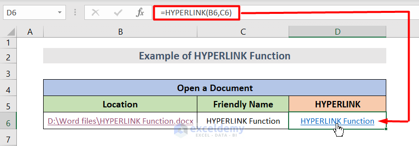
8. Open a Document with HYPERLINK Function
To make a hyperlink that opens a Word document, give the full path to the formula.
=HYPERLINK(“D:\Word files\HYPERLINK function.docx”, “HYPERLINK function”)To open a document, we keep the location in cell B6 and the friendly name in cell C6. And the link to open the document in cell D6. The formula will be
=HYPERLINK(B6,C6) It is now shorter.
What Are the Reasons and Solutions If HYPERLINK Function Is Not Operating?
A non-existent or broken path in the link location argument is the most typical reason for not working a Hyperlink formula.
- If you click a HYPERLINK and the link destination does not open, make sure the link_location is provided in the correct format.
- If an error such as VALUE! or N/A occurs in a cell instead of the link text, the fault is most likely with the friendly_name argument of your Hyperlink formula.
Such problems are most common when friendly_name is returned by another function. For example, if you create a HYPERLINK to the first match using VLOOKUP. If the lookup value is not found within the lookup table, the #N/A error will appear in the formula column. Use the IFERROR function to display an empty string or other user-friendly text instead of the error value to avoid such errors.
Things to Remember
- Excel HYPERLINK function only works with internet URLs. The link location can be a text string wrapped in quotation marks, or a cell reference containing the link as a text string can be supplied.
- An error appears if the path indicated in link_location is no longer available.
- A text, a name, a value, or a cell containing the jump text or value can be used as the friendly_name.
- The cell throws the error instead of the jump text if friendly_name returns an error #VALUE.
Download Practice Workbook
You can download the workbook and practice with them.
Conclusion
Hope this will help you! If you have any questions, suggestions, or feedback, please let us know in the comment section.
<< Go Back to Excel Functions | Learn Excel
Get FREE Advanced Excel Exercises with Solutions!
