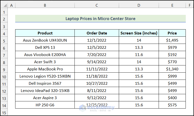
Let’s say we have the Laptop Prices in the Micro Center Store as our dataset. We will use various filters based on cell values to filter the Pivot Table.
Method 1 – Filtering the Pivot Table Using the Search Box Option
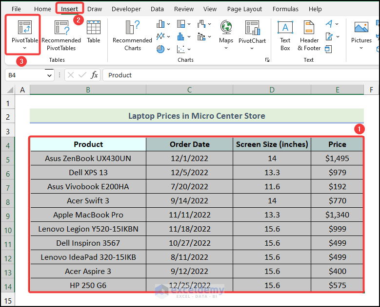
Step 1 – Create a Pivot Table
- Select the entire dataset and go to the Insert tab from Ribbon.
- Select the PivotTable option from the Tables group.
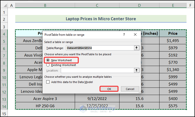
- The PivotTable from table or range dialogue box will appear on your worksheet.
- Choose the New Worksheet option.
- Click OK.
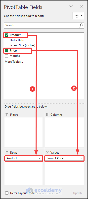
- The PivotTable Fields dialogue box will be available as shown in the following image.
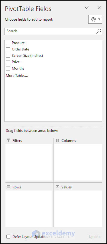
- Drag the Product field to the Rows section.
- Drag the Price field to the Values section.
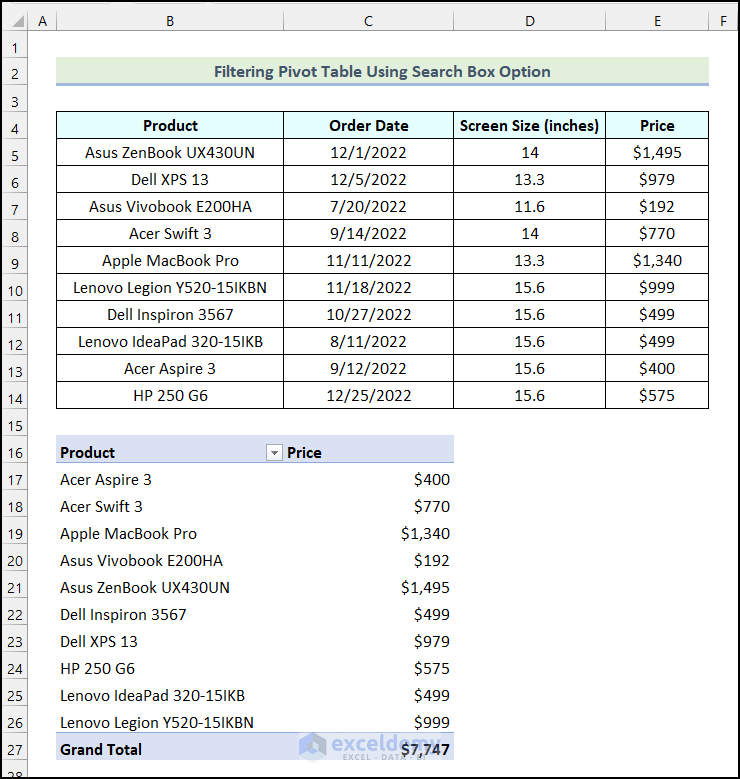
- You will get the following Pivot Table on your worksheet.
Step 2 – Apply the Filter Option in the Pivot Table
- Click on the filter button as marked in the image below.
- Click on the Search Box and type the text based on which you want to filter the Pivot Table. We put “Acer” in the Search Box.
- Click OK.
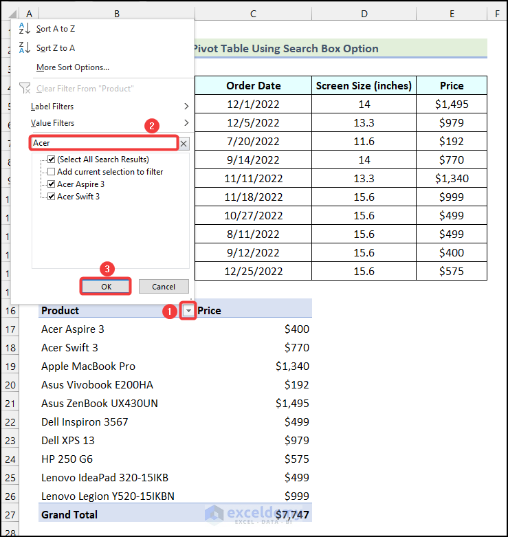
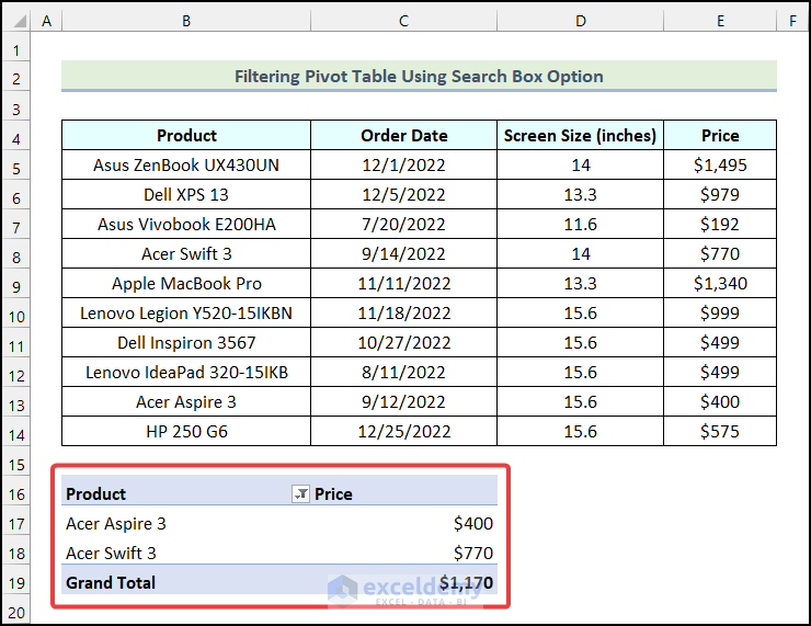
- The Pivot Table will be filtered with all the Products that have Acer in it.
Read More: Excel VBA to Filter Pivot Table Based on Cell Value
Method 2 – Using a Text Value via Label Filters to Filter the Pivot Table
Case 2.1 – Finding Values in a Pivot Table Based on Exact Text
Steps:
- Follow the steps mentioned in Step 1 of the first method to create a Pivot Table.
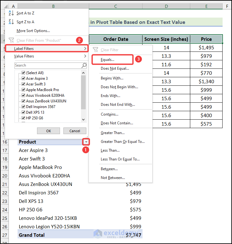
- Click on the filter button as shown in the image below.
- Choose the Label Filters option.
- Select the Equals option.
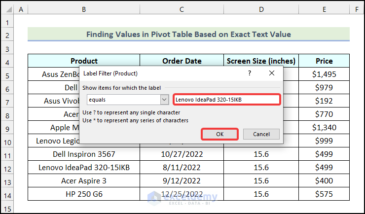
- A dialogue box named Label Filter (Product) will appear on your worksheet.
- Enter the filter text in the marked field as shown below. We inserted “Lenovo IdeaPad 320-15IKB”.
- Click OK.
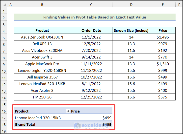
- The Pivot Table will be filtered based on the text that you used as demonstrated in the following picture.
Read More: How to Hide Filter Arrows from Pivot Table in Excel
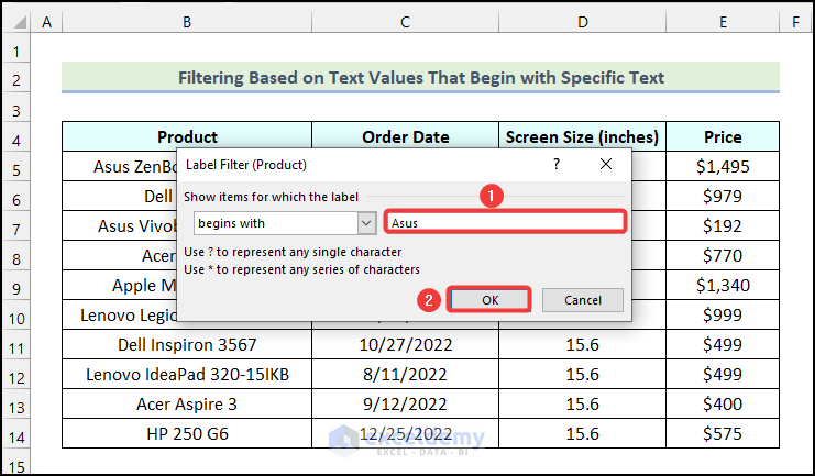
Case 2.2 – Filtering Based on Text Values That Begin with a Specific Text
Let’s say we want to get all the Products that contain Asus.
Steps:
- Use the steps outlined in Step 1 of the first method to create a Pivot Table.
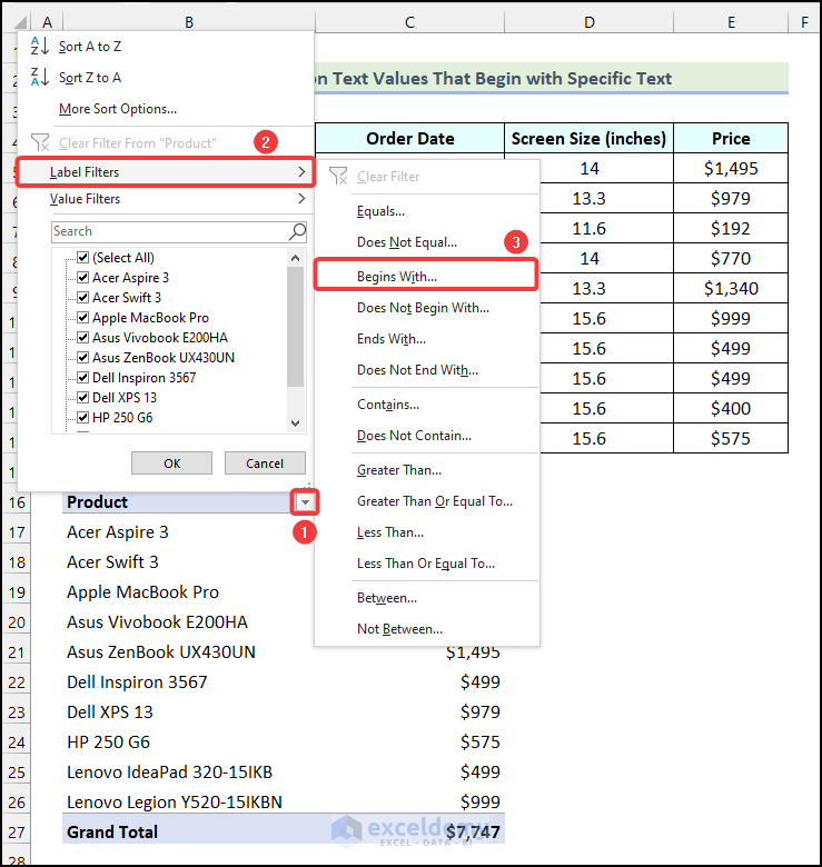
- Click on the filter button as shown in the image below.
- Select the Label Filters option.
- Select the Begins With option.
- A dialogue box named Label Filter (Product) will appear on your worksheet.
- Enter the beginning text. We used Asus.
- Click OK.
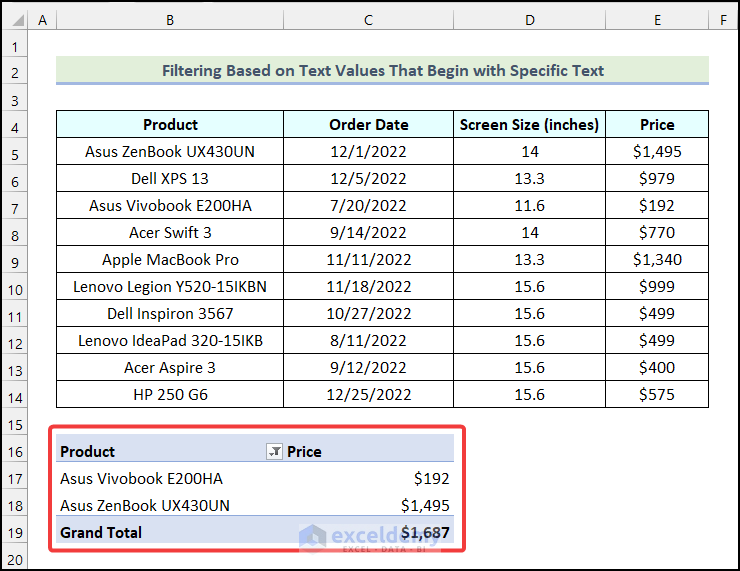
- All the Products from Asus will be available as shown in the image below.
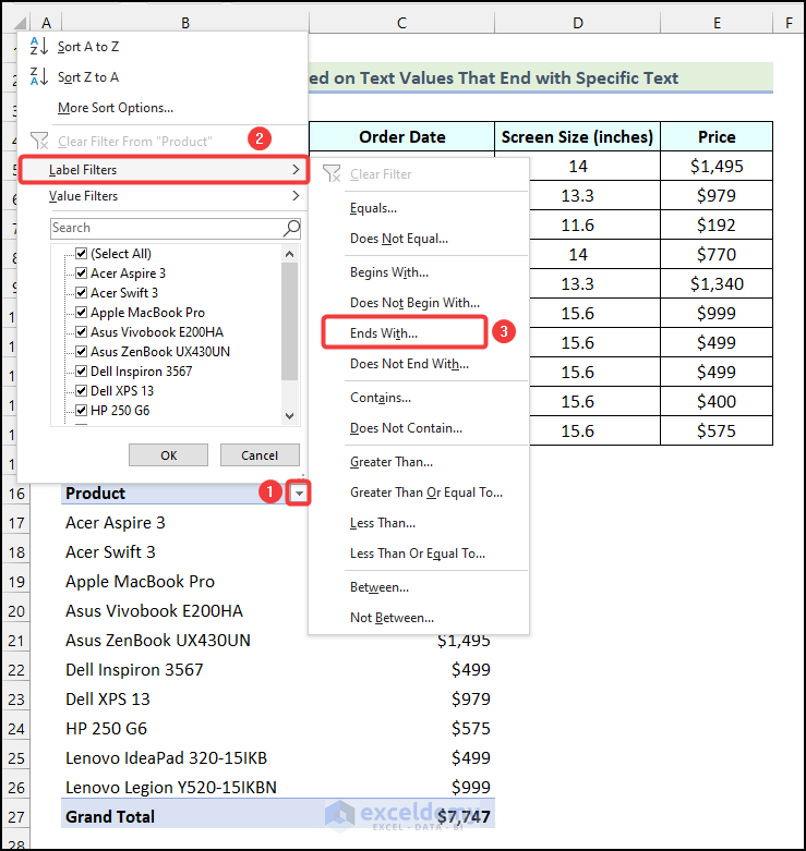
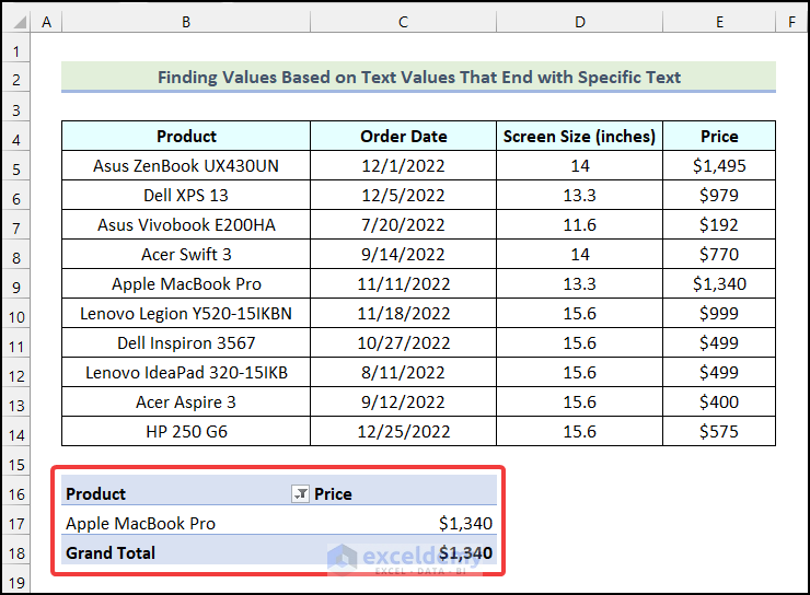
Case 2.3 – Finding Values That End with a Specific Text
Let’s say we want to show the Products that have “Pro” at the end of their name.
Steps:
- Apply the steps discussed in Step 01 of the first method to create a Pivot Table.
- Click on the filter button as shown in the image below.
- Choose the Label Filters option.
- Select the Ends With option.
- A dialogue box named Label Filter (Product) will appear on your worksheet.
- Enter the ending text. We put Pro.
- Click OK.
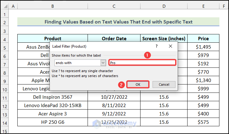
- You will have the list of the Products that have “Pro” at the end of their name.
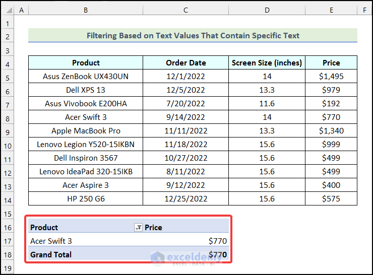
Case 2.4 – Filtering Based on Text Values That Contain a Specific Text
We want to show only the Product that has a text called “Swift” in it.
Steps:
- Use the procedure mentioned in Step 1 of the first method to create a Pivot Table.
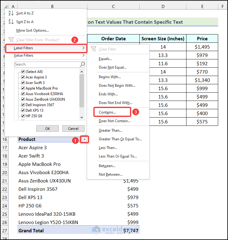
- Click on the filter button as shown in the image below.
- Choose the Label Filters option.
- Select the Contains option.
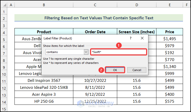
- A dialogue box named Label Filter (Product) will appear on your worksheet.
- Enter the text that should be present inside the Product name. We used “*Swift*”.
- Click OK.
We used Wildcards to define the containing text. “*Swift*” means that any text can be present before and after the word Swift.
You will get the following output on your worksheet.
Method 3 – Filtering a Pivot Table Based on Dates
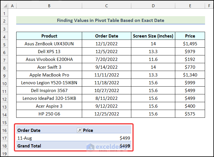
Case 3.1 – Finding Values in Pivot Table Based on an Exact Date
Step 1 – Insert a Pivot Table
- Follow the steps mentioned in Step 1 of the first method to create a Pivot Table.
- While defining the PivotTable Fields, drag the Order Data field to the Rows section and the Price field to the Values section.
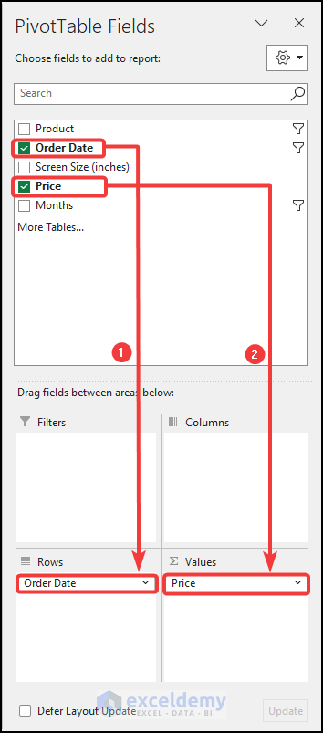
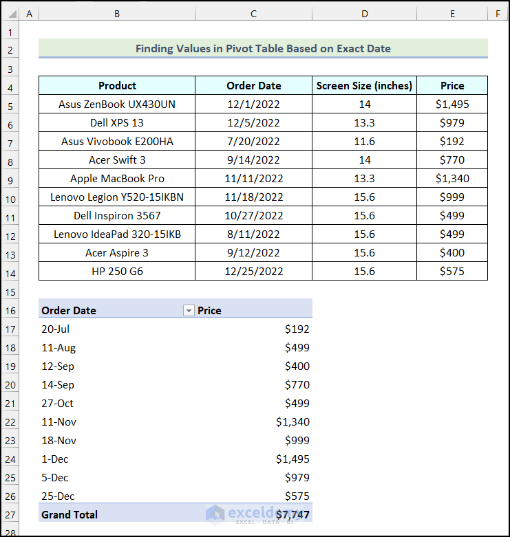
- You will get the following Pivot Table on your worksheet.
Step 2 – Define the Date Filter
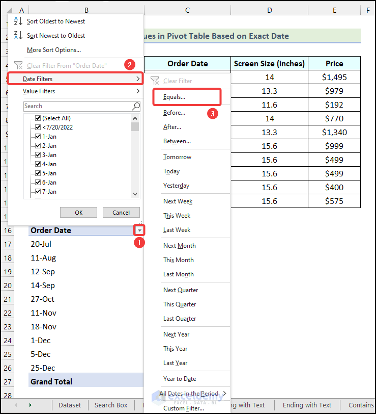
- Click on the filter button as shown in the image below.
- Select the Date Filters option.
- Click on the Equals option.
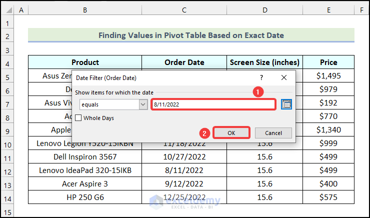
- A dialogue box named Date Filter (Order Date) will appear on your worksheet.
- Enter the date based on which you want to filter the Pivot Table. We used the date 8/11/2022.
- Click OK.
- The Pivot Table will be filtered for only the date 8/11/2022 as demonstrated in the following image.
Case 3.2 – Filtering the Pivot Table Before a Specific Date
Steps:
- Insert a Pivot Table following Step 1 in Case 3.1.
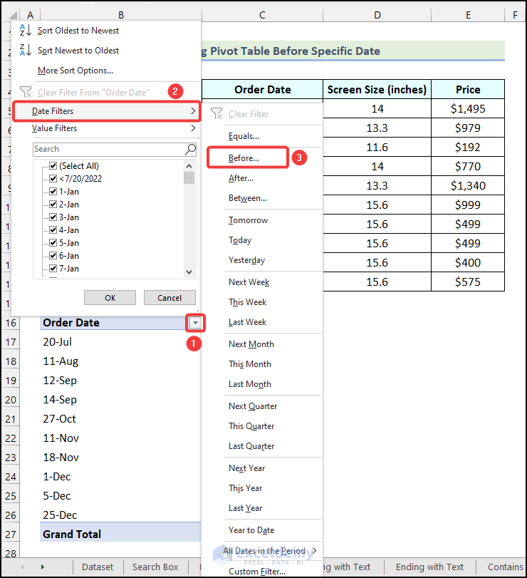
- Click on the filter button as shown in the image below.
- Select the Date Filters option.
- Choose the Before option.
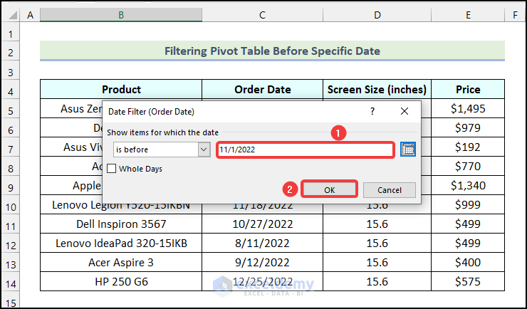
- A dialogue box named Date Filter (Order Date) will be available on your worksheet.
- Enter the date based on which you want to filter the Pivot Table. We used the date 11/1/2022.
- Click OK.
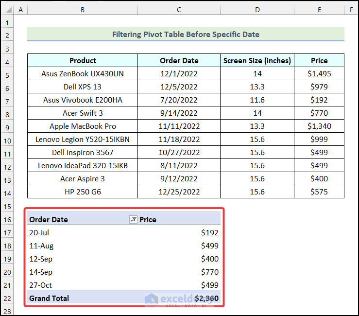
- The Pivot Table will show the “Order Dates” that are before the date 11/1/2022 as shown in the following picture.
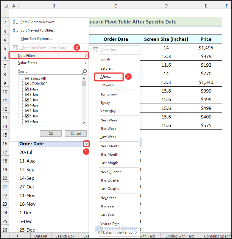
Case 3.3 – Finding Values in a Pivot Table After a Specific Date
Steps:
- Follow the steps mentioned in Step 1 of Case 3.1 to insert a Pivot Table.
- Click on the filter button as shown in the following picture.
- Choose the Date Filters option.
- Select the After option.
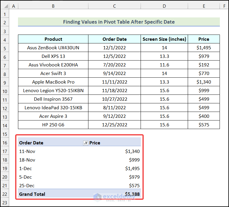
- A dialogue box named Date Filter (Order Date) will be available on your worksheet.
- Enter the date based on which you want to filter the Pivot Table. We used the date 11/1/2022.
- Click OK.

- The Pivot Table will display the “Order Dates” that are after the date 11/1/2022 as demonstrated in the image below.
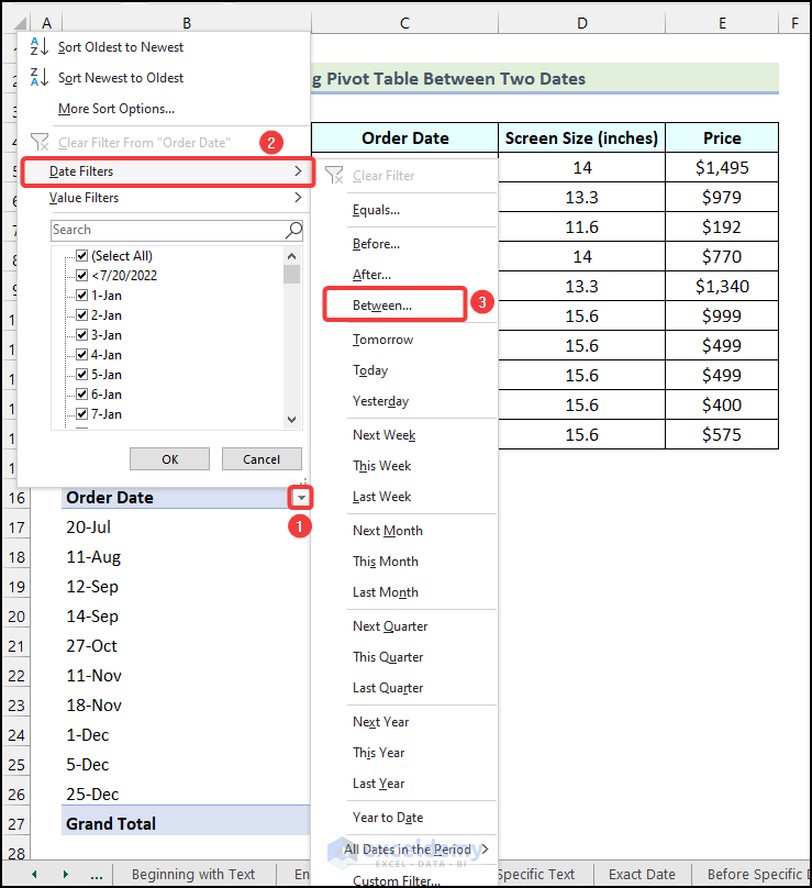
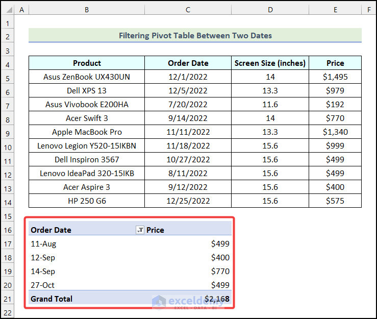
Case 3.4 – Filtering a Pivot Table Between Two Dates
Steps:
- Follow Step 1 of Case 3.1 above to insert a Pivot Table.
- Click on the filter button as shown in the following image.
- Choose the Date Filters option.
- Select the Between option.
- A dialogue box named Date Filter (Order Date) will pop up.
- Insert the starting date and the ending date based on which you want to filter the Pivot Table. We used the dates 8/1/2022 and 10/31/2022, respectively.
- Click OK.
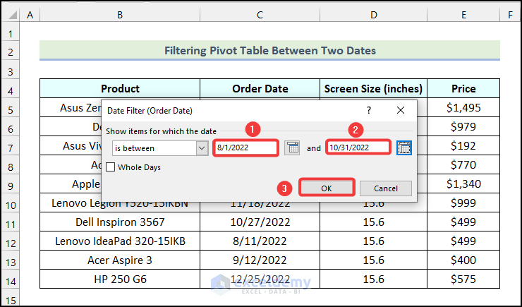
- You will have the “Order Dates” between the starting date and the ending date as shown in the following image.
Read More: Excel VBA Pivot Table to Filter Between Two Dates
Method 4 – Utilizing a Numerical Value for Filtering a Pivot Table
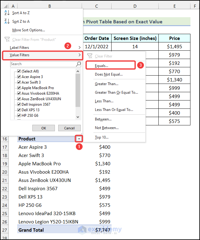
Case 4.1 – Finding Values in a Pivot Table Based on the Exact Value
We want to obtain the name of the Product that has a Price equal to $979.
Steps:
- Use the steps outlined in Step 1 of the first method to create a Pivot Table.
- Click on the filter button as shown in the image below.
- Choose the Value Filters option.
- Select the Equals option.
- A dialogue box named Value Filter (Product) will appear.
- Choose the Price option as marked in the image below.
- Insert the exact value based on which you want to filter the Pivot Table. We used 979.
- Click OK.
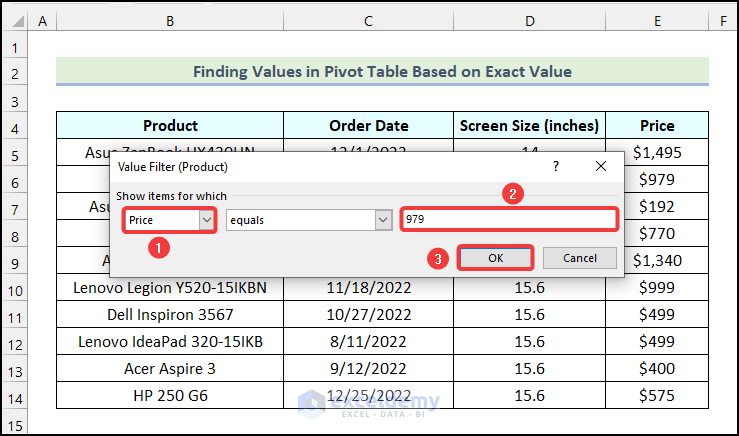
- You will get the name(s) of the Product with a Price of $979 as shown in the following picture.

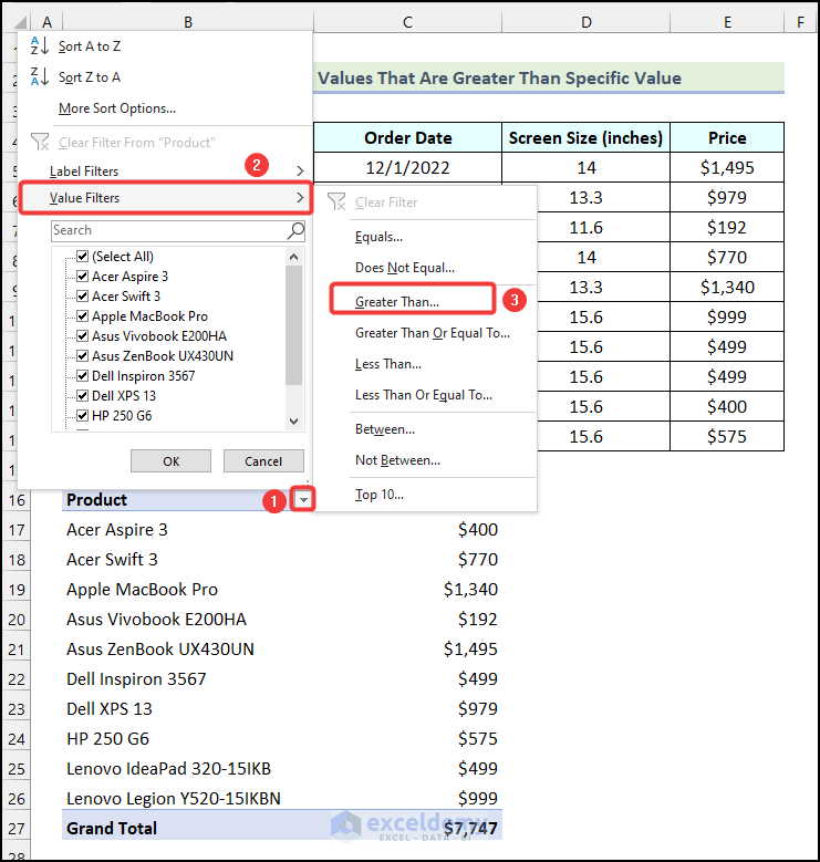
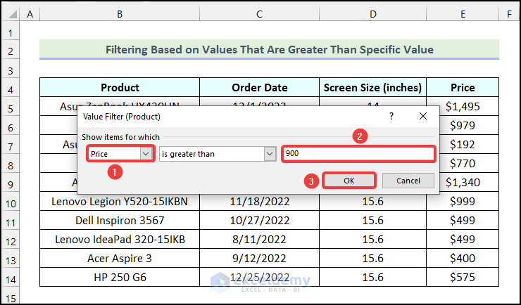
Case 4.2 – Filtering Based on Values That Are Greater Than a Specific Value
We want to show the names of the Products that have Prices greater than $900.
Steps:
- Use the steps outlined in Step 1 of the first method to create a Pivot Table.
- Click on the filter button as shown in the image below.
- Choose the Value Filters option.
- Select the Greater Than option.
- A dialogue box named Value Filter (Product) will appear.
- Select the Price option as marked in the image below.
- Insert the value based on which you want to filter the Pivot Table. We used 900.
- Click OK.
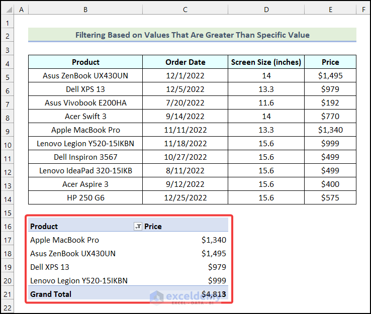
- You will get the name of the Products that have a Price greater than $900.
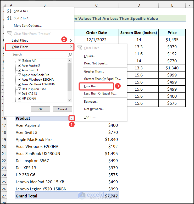
Case 4.3 – Finding Values in a Pivot Table That Are Lower Than the Specific Value
Steps:
- Apply Step 1 of the first method to create a Pivot Table.
- Click on the filter button as shown in the image below.
- Choose the Value Filters option.
- Select the Less Than option.
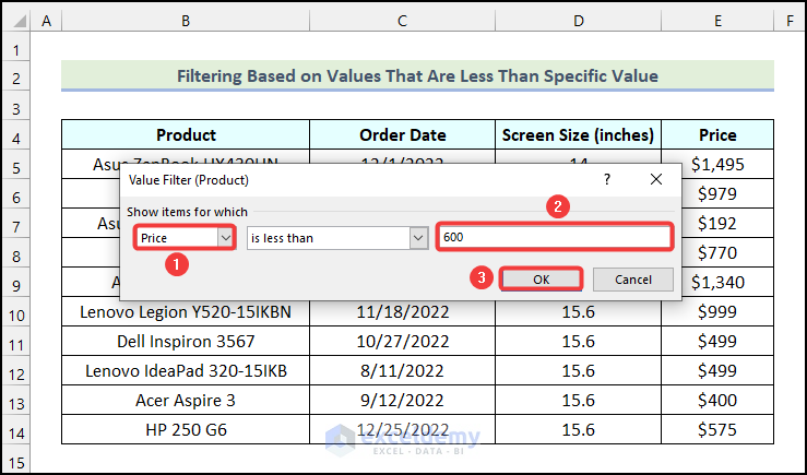
- A dialogue box named Value Filter (Product) will open.
- Select the Price option as marked in the image below.
- Enter the value based on which you want to filter the Pivot Table. We used “600”.
- Click OK.
- You will have the name of the Products that have a Price less than $600.

Case 4.4 – Filtering a Pivot Table Between Two Values
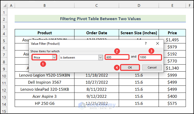
Let’s find the names of the Products with a Price range from $600 to $1,000.
Steps:
- Follow Step 1 of the first method to create a Pivot Table.
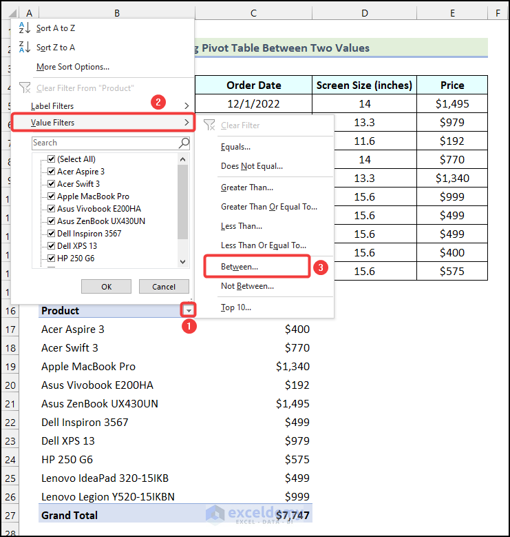
- Click on the filter button as shown in the image below.
- Choose the Value Filters option.
- Select the Between option.
- A dialogue box named Value Filter (Product) will open.
- Select the Price option as marked in the image below.
- Enter the two values based on which you want to filter the Pivot Table. We used “600” and “1000” as the filter range values.
- Click OK.
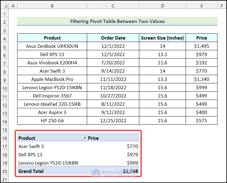
- Here are the results.
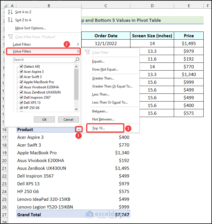
Case 4.5 – Finding the Top and Bottom 5 Values in a Pivot Table
Steps:
- Follow the instructions in Step 1 of the first method to create a Pivot Table.
- Click on the filter button as shown in the image below.
- Select the Value Filters option.
- Choose the Top 10 option.
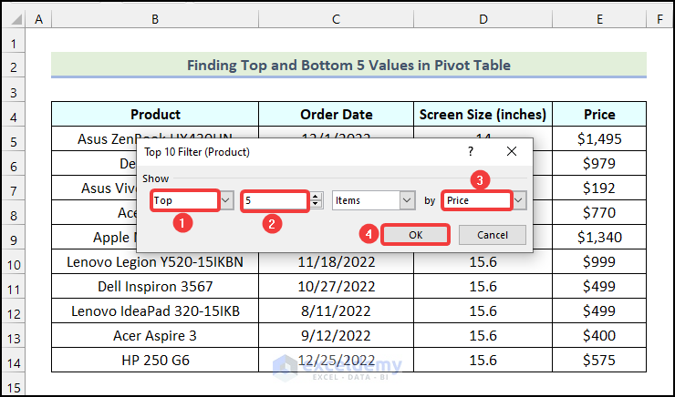
- A dialogue box named Value Filter (Product) will open.
- Select the Top option as marked in the image below.
- Enter 5 as we need the top 5 values.
- Choose the Price option as shown in the following picture.
- Click OK.
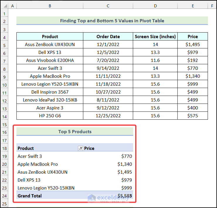
- Here are the results.
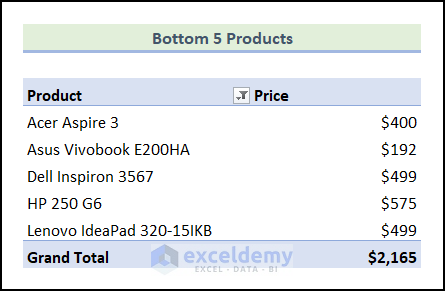
- You can also find the bottom 5 values by selecting the Bottom option in the Value Filter (Product) dialogue box.
Method 5 – Using a Slicer to Filter Data Based on Cell Value
Steps:
- Follow Step 1 of Method 1 to create a Pivot Table.
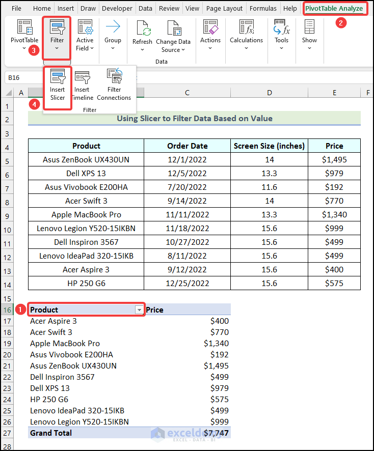
- Click on any cell of the created Pivot Table to access the PivotTable Analyze tab.
- Select the Filter option.
- Choose the Slicer option from the drop-down.
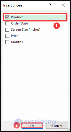
- The Insert Slicers dialogue box will appear.
- Check the Product option in the Insert Slicers dialogue box.
- Click OK.
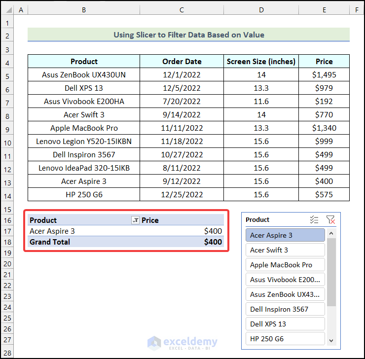
- A Slicer will be added to your worksheet as shown in the following picture.
- Choose any Product from the Slicer to filter the Pivot Table based on your selection. We selected the “Acer Aspire 3” option.

You will get the results.
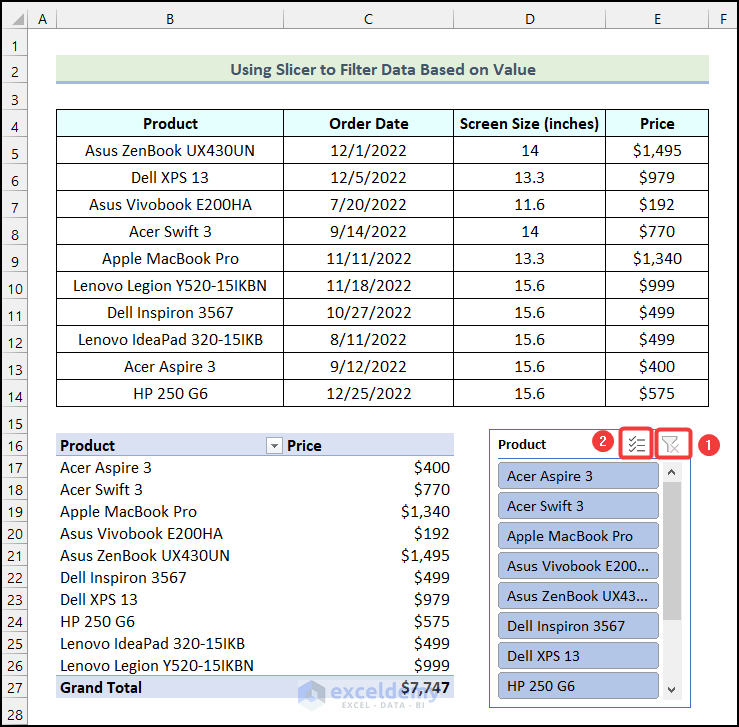
Follow these steps if you want multiple criteria for Slicers.
- Click on the Clear Filter option in the Slicer as marked in the following image.
- Click on the Multi-Select option in the Slicer.
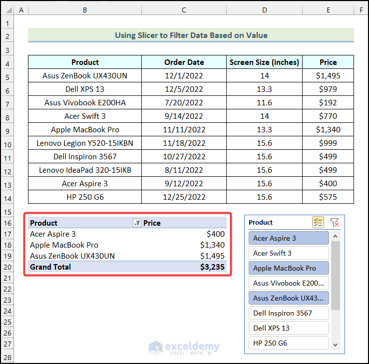
- Select the names of the Products based on which you want to filter the Pivot Table. We have chosen Acer Aspire 3, Apple MacBook Pro, and Asus ZenBook UX430UN.
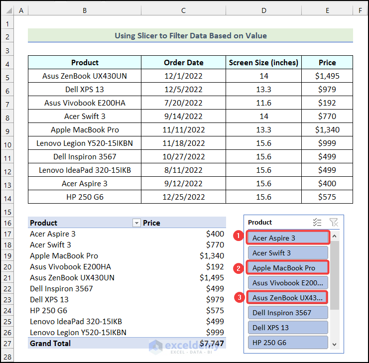
The Pivot Table will be filtered based on your selections as shown in the image below.
Method 6 – Inserting a Timeline to Filter Data in a Pivot Table
The Timeline feature doesn’t work with the texts and numbers. It only works with dates and times.
Steps:
- Follow Step 1 of Method 3 to create a Pivot Table.
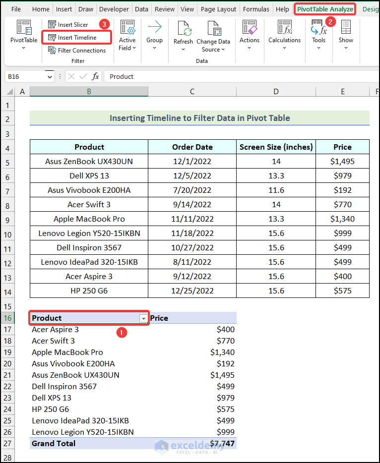
- Click on any cell of the created Pivot Table to access the PivotTable Analyze tab.
- Choose the Insert Timeline option from the Filter group.
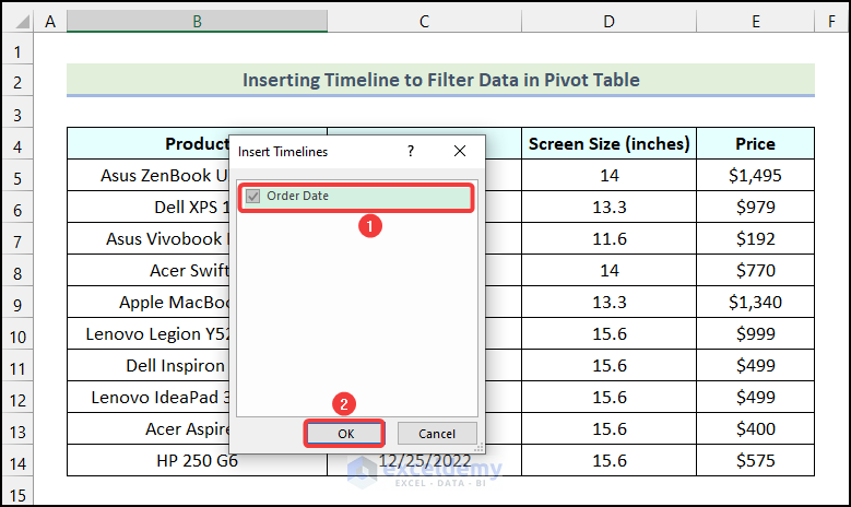
- The Insert Timelines dialogue box will open on your worksheet.
- Check the field for the Order Date option.
- Click OK.
- A Timeline will be added to your worksheet as shown in the following picture.
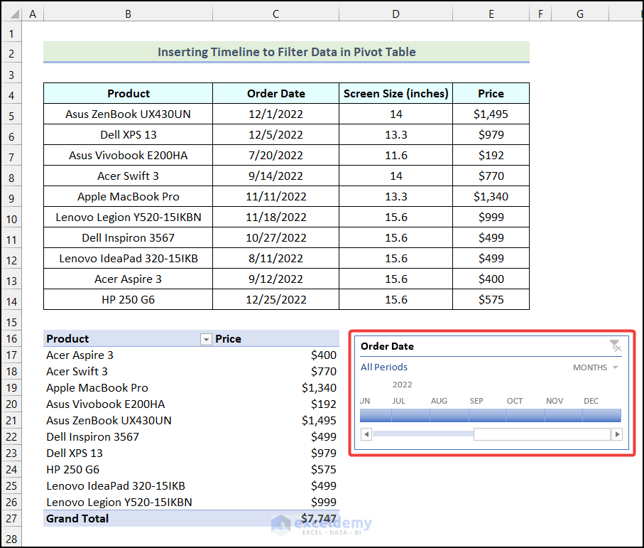
- Select the range of months based on which you want to filter the Pivot Table. We selected the months of August, September, and October.
- The Pivot Table will be filtered based on your selected months from the Timeline as demonstrated in the following picture.

Read More: How to Create a Timeline in Excel to Filter Pivot Table
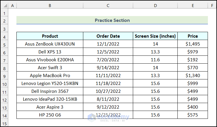
Practice Section
In the Excel Workbook, we have provided a Practice Section in the worksheet.
Download the Practice Workbook
<< Go Back to Pivot Table Filter | Pivot Table in Excel | Learn Excel
Get FREE Advanced Excel Exercises with Solutions!
