The timeline slicer helps filter dates in the pivot table.
Step 1 – Convert the Dataset into a Table
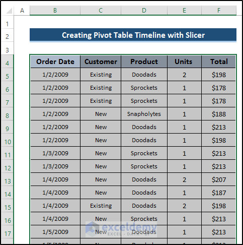
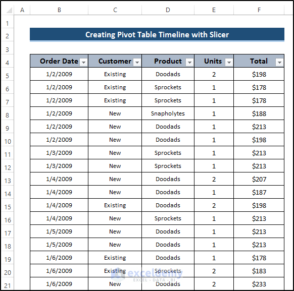
- Select the entire dataset to create a table.
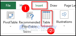
- Go to the Insert tab.
- Select Table in Tables.
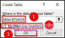
- In the Create Table dialog box, you will see your dataset converted into a table.
- Check on My table has headers.
- Click OK.
This is the output.
Step 2 -Convert the Table into a Pivot Table
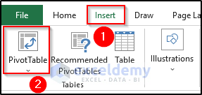
- Go to the Insert tab.
- Select PivotTable in Tables.
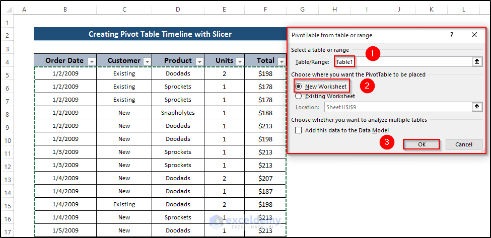
- In the PivotTable from table or range dialog box, select Table1 in Table/Range.
- Select New Worksheet.
- Click OK.
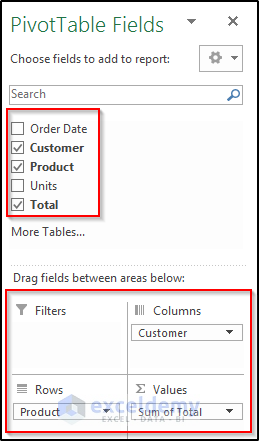
- In the Pivot Table Fields dialog box, select Customer, Product, and Total.
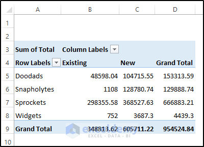
- Drag Customer to Columns, Product to Rows, and Sum of Total to Values.
This is the output.
Step 3 – Insert a Timeline Slicer to Filter the Pivot Table
- Click the pivot table.
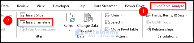
- Go to Pivot Table Analyze.
- Select Insert Timeline in Filter.
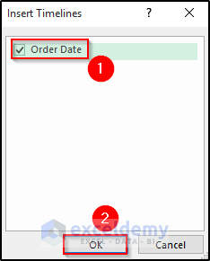
- In the Insert Timelines dialog box, check Order Date.
- Click OK.
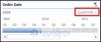
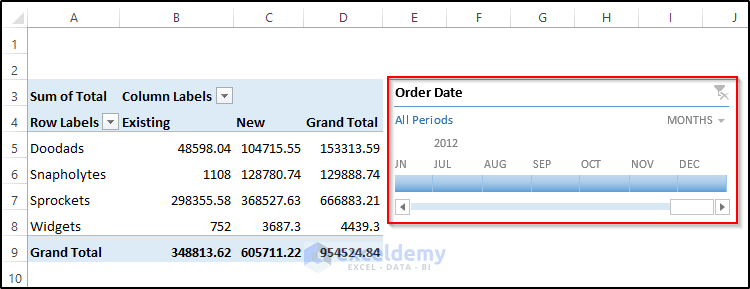
You will see the following pivot table timeline slicer with a date range from 2009 to 2012.
By default, Excel sets the timeline in months.
- Change the date range from monthly to quarters by clicking the down arrow sign.
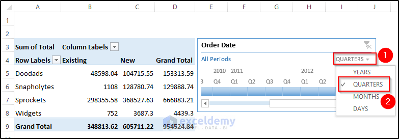
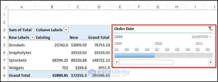
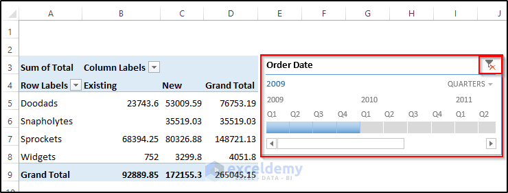
- To see the pivot table for 2009, select the four quarters in 2009.
You will see the filtered values of 2009:
How to Clear the Filter from a Timeline in Excel
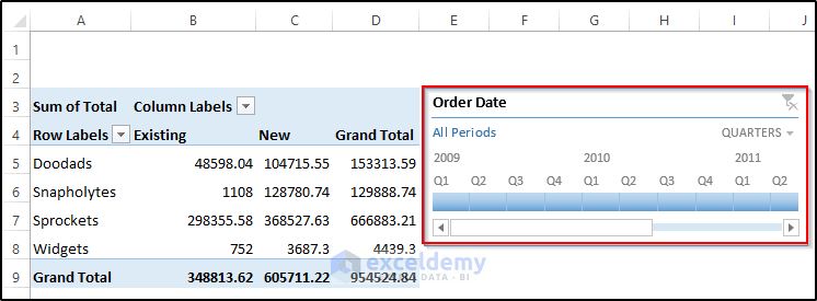
- Click the Clear Filter option at the top right corner of the timeline.
- It shows values from 2009 to 2012.
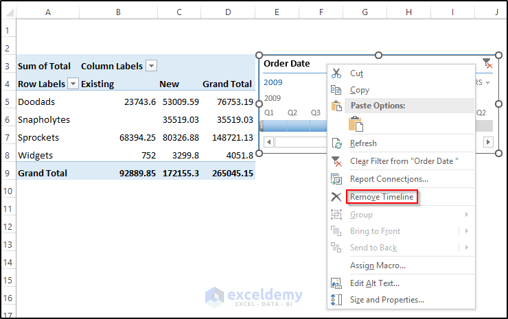
How to Remove a Pivot Table Timeline in Excel
- Right-click the timeline.
- Select Remove Timeline.
The timeline is removed.
Things to Remember
- The timeline only takes values when there is a field formatted as date.
Download Practice Workbook
Download the practice workbook.

