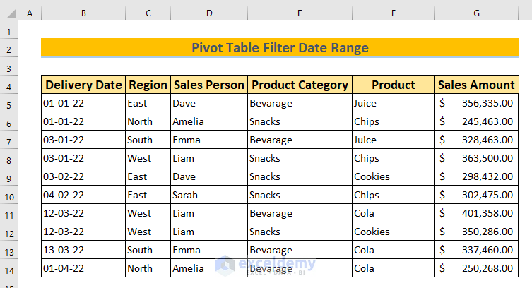
Suppose we have a dataset of a company’s sales having Delivery Date, Region, Salesperson, Product Category, Product and Sales Amounts. We’ll use a pivot table to filter the date ranges.
Method 1 – Using Check Boxes to Filter a Date Range in an Excel Pivot Table
Steps:
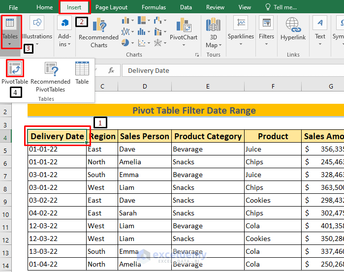
- Select any cell in your data range. You can’t have any blank columns or rows within your dataset.
- Go to the Insert tab, select Tables, and choose PivotTable.
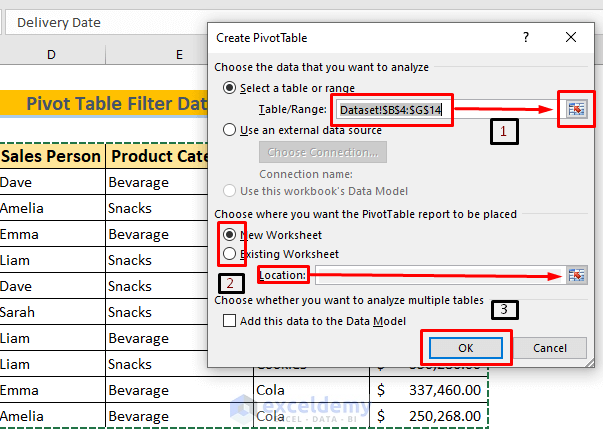
- The Create PivotTable dialogue box will open.
- Your table or range will be automatically selected if you have selected it initially. Otherwise, select it using the Select button shown with an arrow in the image below.
- If you want to work in the Existing Worksheet, check that option and use the Location button to place where the table will go.
- If you want to work on a New Worksheet, check that option and press OK.
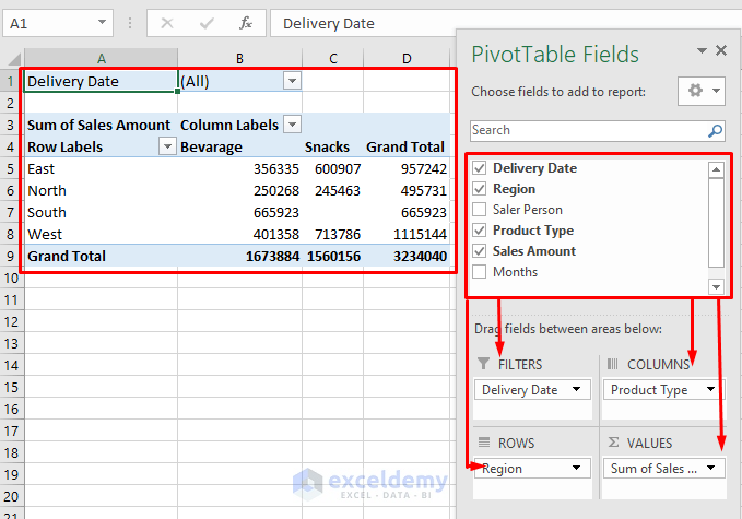
- The PivotTable Fields dialog box will open. It will have all Fields from your dataset’s Column Headings.
- There are four Areas: Filters, Columns, Rows, Values. You can drag any Field to any of the Areas.
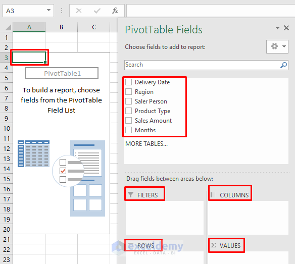
- Drag Delivery Date to FILTERS.
- Suppose we want to find out the relationship between Product Type and Region. Drag them to Column & Row or vice versa.
- We put the Sales Amount in the Value Area to triangulate it with Product Type and Region.
- Excel will create the pivot table at the designated location.
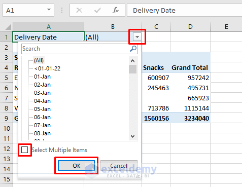
- Click on the drop-down menu beside Delivery Date.
- Click on any date that you want to Filter.
- To select multiple dates, click on Select Multiple Items then make your selection.
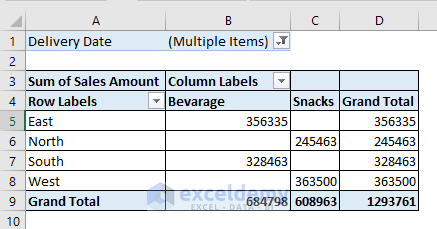
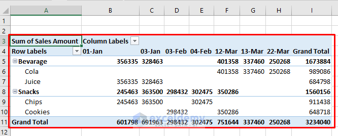
- We have selected 01-Jan to 04-Jan.
- Click OK.
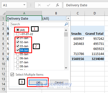
- Your Pivot Table will contain only values from 01-Jan to 04-Jan. You can also select discrete dates just by clicking on them.
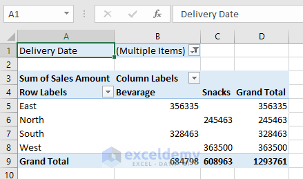
- We have removed gridlines and selected all borders for the Pivot Table.
Method 2 – Using an Excel Pivot Table to Filter a Date within a Specific Range
Steps:
- Create a Pivot Table with the dataset following the same procedures as in Method 1.
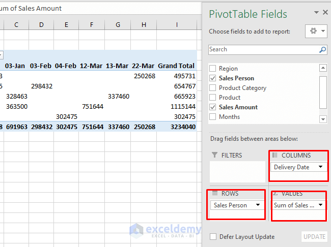
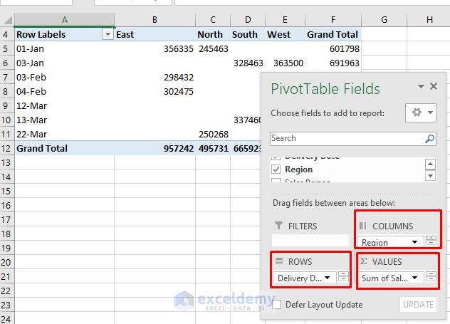
- Drag the Delivery Date field to Column. If we want to see its relationship with Salesperson and Sales Amount, drag both to Row and Values.
- We will get a Pivot Table.
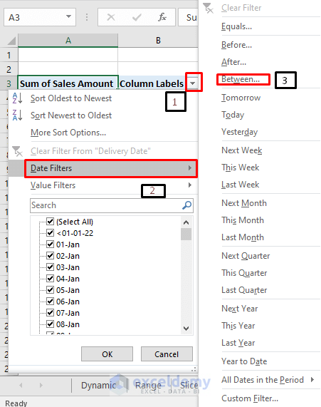
- To filter with a range of dates, click on the Column Drop-Down beside Column Labels.
- Select Date Filters.
- Select Between.
- You can select any other desired Filters like This Month, Last Week, Last Year, etc. which are called Dynamic Dates and we have shown them in a different section.
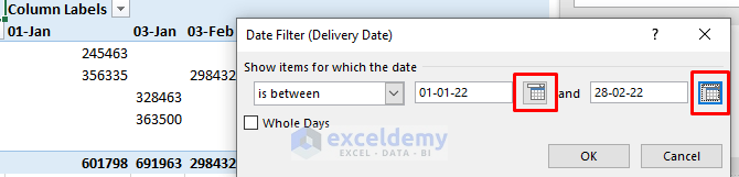
- Upon selecting Between, the Date Filter dialogue box will open.
- Select the range of dates you want to Filter.
- We have selected is between, 01-01-2022, and 28-02-2022.
- Our Pivot Table will show data only with the filtered range of dates.
Method 3 – Using Date Filters Within an Excel Pivot Table
Steps:
- We have put Delivery Date in Rows, Region in Column, and Sales Amount in Values.
- This Pivot Table will show us the Sales Amount for each Region per Delivery Date.
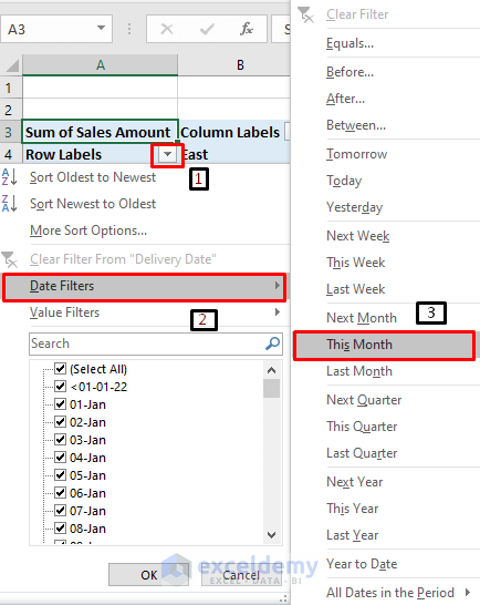
- To find the region-wise Sales Amount for a specific time only, select the Row Labels Drop-Down.
- Select the Date Filters.
- Select any desired Dynamic Date. We have selected This Month.
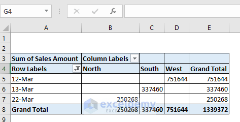
- This will show the Sales Amount for This Month.
- After removing gridlines and selecting all borders for our data cells, we will get our desired Pivot Table.
Read More: Excel Pivot Table Date Filter Not Working
Method 4 – Filtering the Date Range in an Excel Pivot Table with Slicers
Steps:
- We have created a Pivot Table having Delivery Date in Column Headings and Product Type and Product in Row Headings.
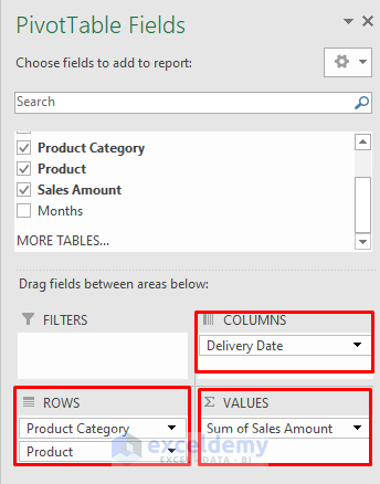
- We input Sales Amounts in Values Area. You can select your desired Field, and can drag multiple fields in a single area to make a more detailed Pivot Table.
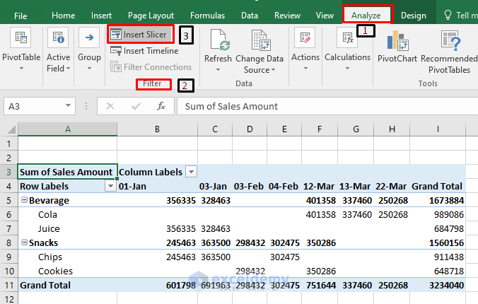
- Go to Analyze, select Filter, and choose Insert Slicer.
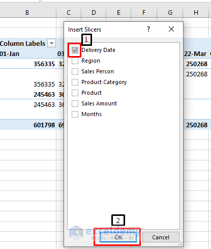
- The Insert Slicers dialogue box will show up. Select the Field you want to filter. We have selected Delivery Date as we want to filter with dates.
- Press OK.
- The Delivery Date box will open up. You can select any date from here for filtering.
- To select multiple dates, select the checkbox at the top-right, then select multiple dates.
- We have selected 01-Jan, 04-Feb, and 13-Mar for filtering the Pivot Table.

- The Pivot Table will show us the data of the above 3 selected dates and we will have our desired Pivot Table.
Method 5 – Using the Pivot Table to Filter a Date Range with Timelines in Excel
Steps:
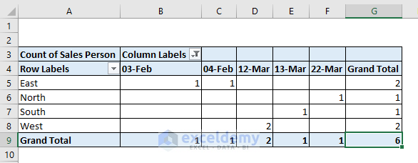
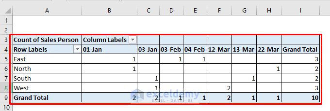
- We have created a Pivot Table using Delivery Date in Column Headings, Region as Row Headings, and Salesperson as Value.
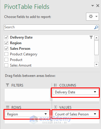
- The Values area inputs everything as a numeric value. So, it counted each Salesperson to be One.
- Go to Analyze, select Filters, and choose Timeline.
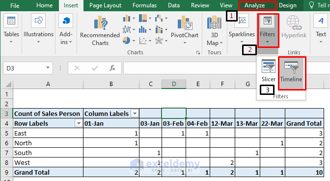
- The only option available here is Delivery Date. Select it in the box, and press OK.
- Move the Blue bar left and right to select your desired Timeline. We have selected FEB and MAR.
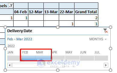
- Excel will show us our desired Pivot Table with Sales from Feb and Mar.
Read More: How to Create a Timeline in Excel to Filter Pivot Table
Download the Practice Workbook

