Excel Funnel Chart

Here’s an example where we presented a sample funnel chart that was created with the help of a previously created stacked chart.

How to Create a Funnel Chart in Excel

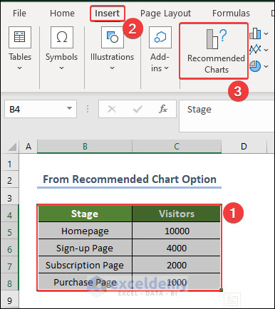
Method 1 – Funnel Chart From Recommended Charts

• Select the range of cell B4:C8.
• Go to Insert and choose Recommended Charts.

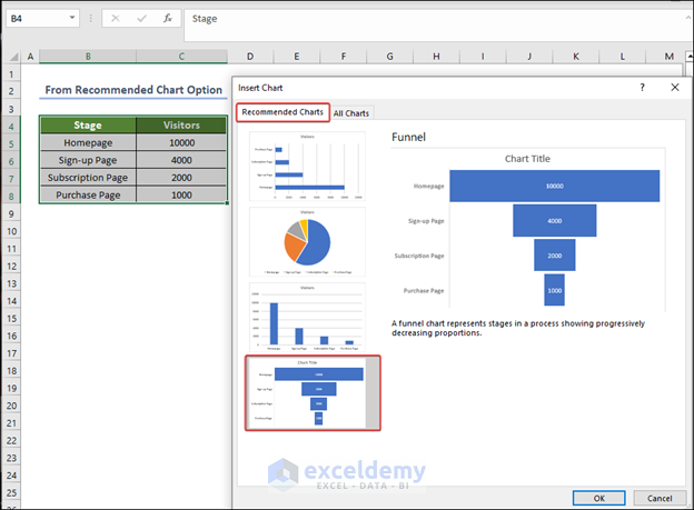
• You’ll get a dialog window.
• Find the funnel-shaped chart in the list on the left.
• Select the chart and click OK.

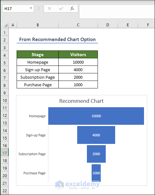
• The chart is now present in the worksheet.

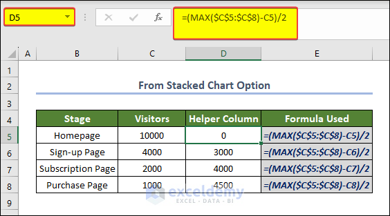
Method 2 – Funnel Chart from a Stacked Chart

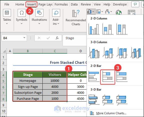
• Enter the following formula in the E5.

• Hit Enter and drag the Fill Handle to cell D8. These are the values that are going to help us convert a simple stacked chart to a funnel chart.

• Go to the Insert tab and select Chart then choose 2d- Stacked Bar chart.

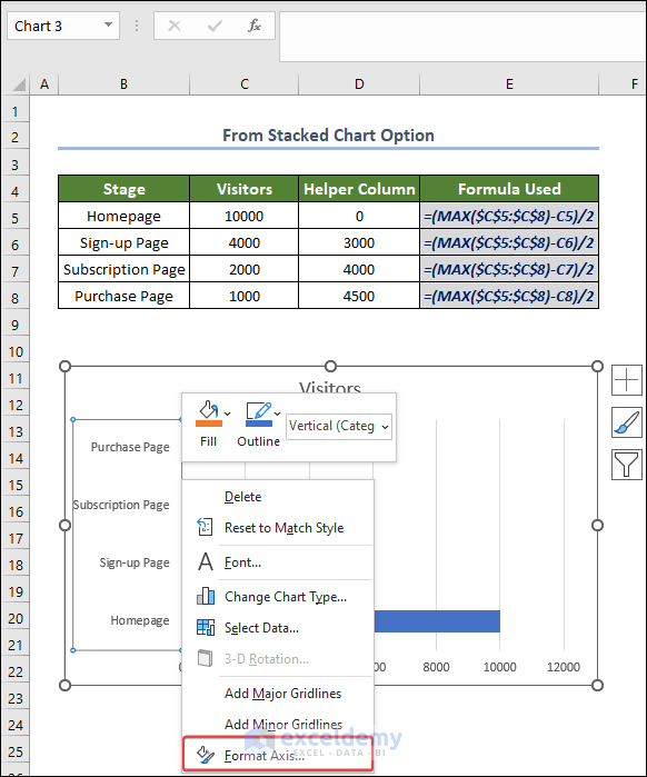
• A chart is now present in the worksheet.
• Right-click on the axis and select Format Axis.

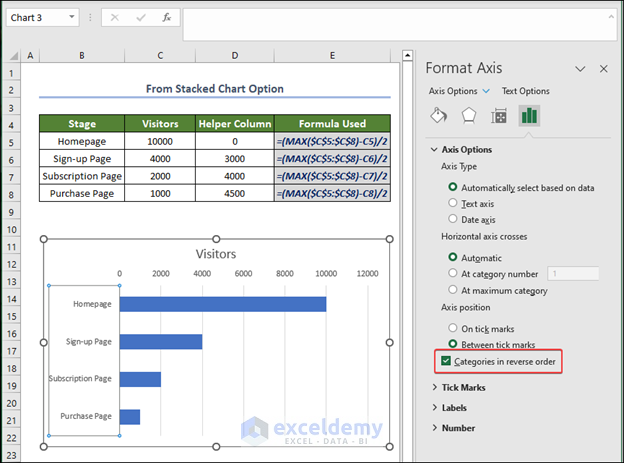
• Go to the rightmost tab in the panel and select the Categories in the reverse order check box.
• The axis values are now reversed.

• Add another column of values to the existing table by selecting D4:D8 in the saved data ranges.
• Click OK.

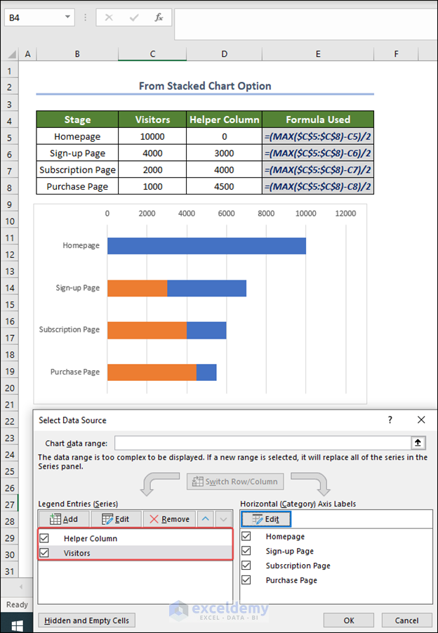
• After adding the data to the worksheet, we will see that there is new data added on top of the existing dataset present in the plot.

• Select the new dataset and right-click on it.
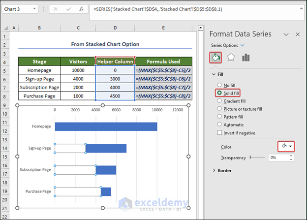
• From the context menu, select Format Data Series.

• In the Format Data Series window, select the Solid fill option in Fill.
• Choose white as the color.

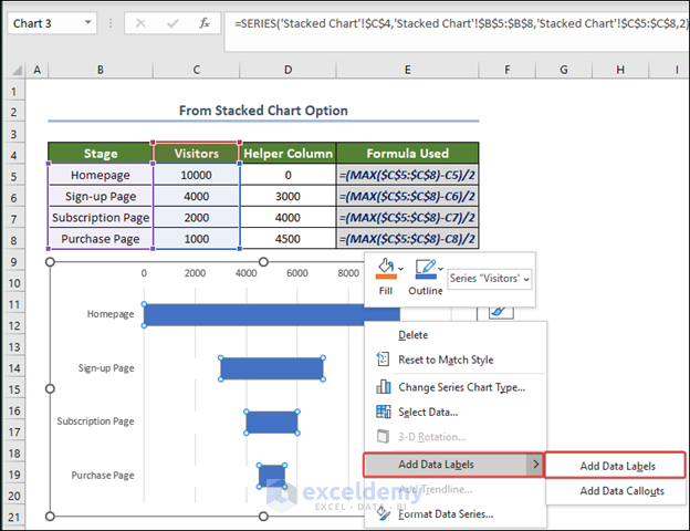
• We can change the color of the text inside the chart by right-clicking on it and then selecting Add Data Labels.
• Choose Add Data Labels

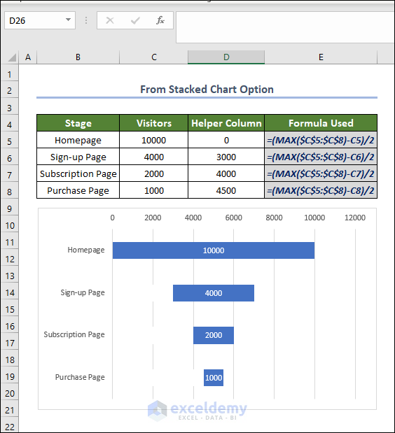
• The chart looks like a funnel.

Method 3 – 3-Dimensional Excel Funnel Chart

• Add a stacked chart to the worksheet.
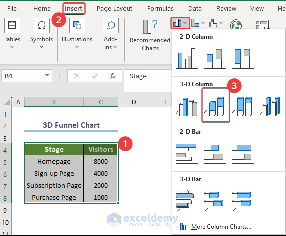
• Select B4:C8, and then go to the Insert tab.
• Choose Insert Column or Bar Chart.
• Choose 3D-Stacked Chart.

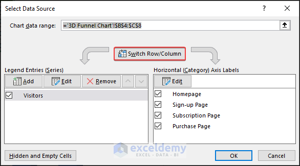
• Change the data row and column serial in the Select Data Source by clicking on the Switch Row/Column.
• Click OK.

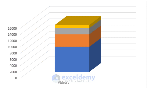
• All of the data is now shown in one column.

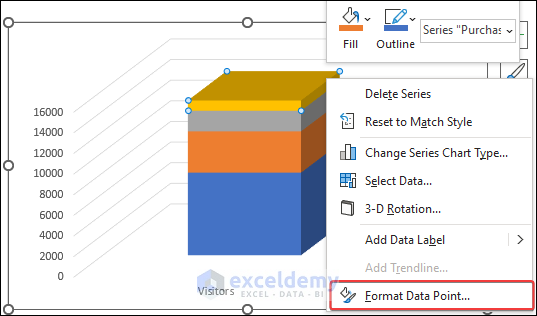
• Click on the data series and, from the context menu, select Format Data Point.

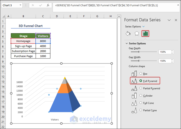
• In the format data point window, select Full Pyramid in the Column Shape
• The column shape is now shifted to the pyramid shape.

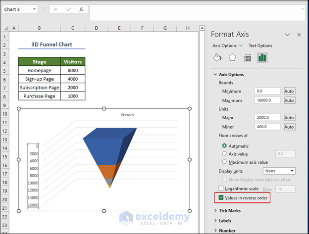
• Right-click on the Y-Axis and then select Format Axis.

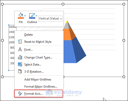
• In the Format Axis window, check Values in the reverse order. The pyramid-shaped chart will be reversed.

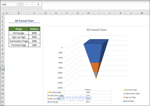
• After some modification, the 3D funnel chart will take the final form shown below.

Things to Remember

Data Setup: Organize your data in a table format with clear headings. The first column should represent the stages or steps, and the subsequent columns should contain the values corresponding to each stage.

Data Order: Make sure your data is sorted in descending order depending on the values. The highest value should be at the top (the first stage), and the values should decrease progressively as you move down the stages.

Select Data: When inserting the funnel chart, ensure that you have selected the correct data range, including both the stage names and the corresponding values.

Chart Type Selection: Choose the right funnel chart type based on your data. Excel offers different funnel chart variations, such as the basic funnel chart or the stacked funnel chart. Select the one that best suits your data representation.

Data Labels: Include data labels on the chart to display the exact values for each stage. This helps readers understand the numbers accurately.

Title and Axis Labels: Provide a clear and descriptive chart title, and label the horizontal axis with appropriate stage names. This makes the chart easy to interpret.

Colors: Choose a visually appealing color scheme for your funnel chart. Use consistent colors or shades to distinguish between different stages.

Formatting: Format the chart elements to make them visually appealing. You can adjust the font size, colors, borders, and other chart properties to enhance its appearance.

Tooltip: Add a tooltip to the chart labels if there is low space for displaying all the data labels. This way, users can hover over the chart to see the values.

Axis Scaling: Ensure that the axis scaling is appropriate and does not distort the representation of the data. The width of each stage should accurately reflect the proportion of values between stages.

Data Validation: Double-check your data for accuracy before creating the chart. Any mistakes in the data can lead to incorrect visualizations.

Chart Placement: Choose the right location to place your funnel chart within the worksheet or the dashboard to make it more effective and visually integrated.

Frequently Asked Questions

What is a funnel chart for?

A funnel chart in Excel visualizes data that undergoes a progressive reduction through different stages. It represents a series of steps, illustrating how the values decrease as you move from one stage to the next. Funnel charts are commonly employed in sales, marketing, website conversions, lead generation, and event registrations to analyze and optimize processes. They help identify drop-offs, conversion rates, and bottlenecks in various workflows, aiding in data-driven decision-making. With clear visuals, funnel charts offer insights into the efficiency and effectiveness of processes, making them valuable tools for data analysis and performance tracking in Excel.

Can you create a stacked funnel chart in Excel?

Excel does not have a built-in stacked funnel chart option. However, you can create a stacked funnel chart using a workaround by combining a stacked bar chart and a funnel chart. This involves adjusting data and formatting to achieve the desired visual representation.

How many data points do funnel charts require in Excel?

Funnel charts in Excel typically require at least two data points, representing the starting and ending values of the funnel. However, for a more informative visualization, it is recommended to have multiple data points representing each stage’s values along the funnel’s progression. The more data points you have, the more detailed and accurate the funnel chart will be in showcasing the progressive reduction at each stage of the process.

<< Go Back to Excel Charts | Learn Excel