Here’s an example of using the FILTER function for dynamic data retrieval and a chart to accompany it.
Download the Practice Workbook
What Is a Dynamic Excel Chart?
In Excel, the dynamic chart is a special type of chart that updates automatically when one or multiple rows are added or removed from the range or table.
How to Create Dynamic Charts in Excel
There are 3 convenient ways to create dynamic charts in Excel. They are:
- Using an Excel Table.
- Applying a Named Range.
- Using VBA Macros.
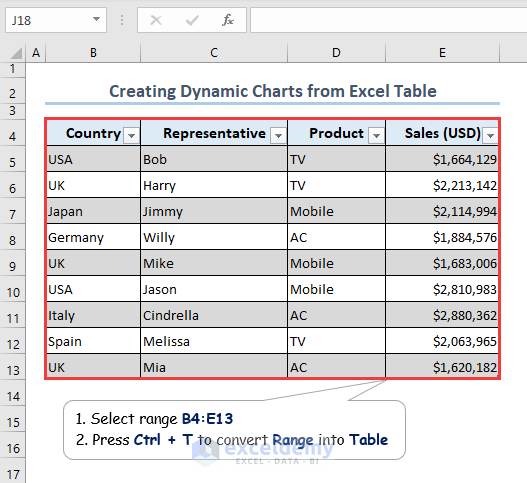
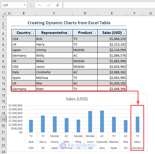
Method 1 – Make Dynamic Charts from an Excel Table
- Select the B4:E13 range.
- Press Ctrl + T to convert the range into a Table.
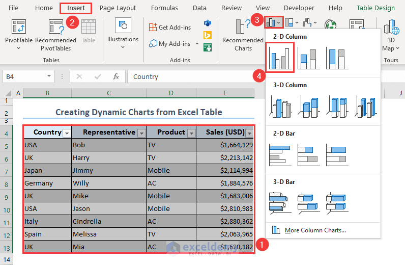
- Select the table.
- Go to the Insert tab, select the Insert Column or Bar Chart command, and choose the 2-D Clustered Column chart type.
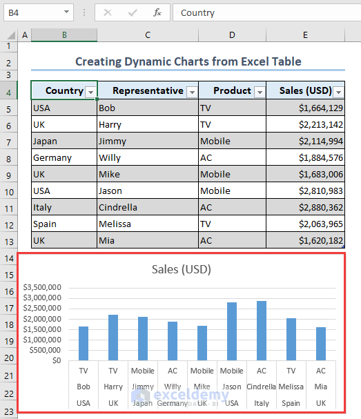
- We get a 2-D Clustered Column chart containing sales of representatives.
- Inserting a row in the B14:E14 range adds the data for Marc in the following chart.
Method 2 – Excel Functions Within a Named Range to Create Dynamic Charts
We will use the OFFSET function to get the grouped range based on relative reference.
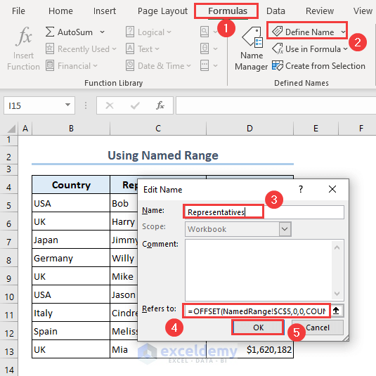
- Go to the Formulas tab and select the Define Name command.
- Type Representatives in the Name field of the Edit Name dialog.
- Insert the following formula containing the OFFSET and COUNTA functions in the Refers to field and hit the OK button.
=OFFSET(NamedRange!$C$5,0,0,COUNTA(NamedRange!$C:$C)-1,1)
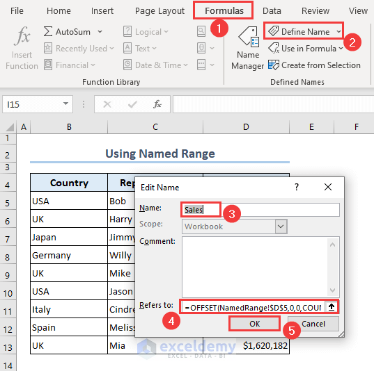
- Make another range Sales for the following formula in the Refers to field.
=OFFSET(NamedRange!$D$5,0,0,COUNTA(NamedRange!$D:$D)-1,1)
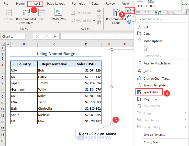
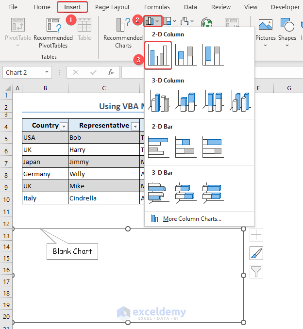
- Go to the Insert menu.
- Click on the Insert Column and Bar Chart command.
- A blank chart appears.
- Right-click on the blank chart.
- Select the Select Data option from the context menu.
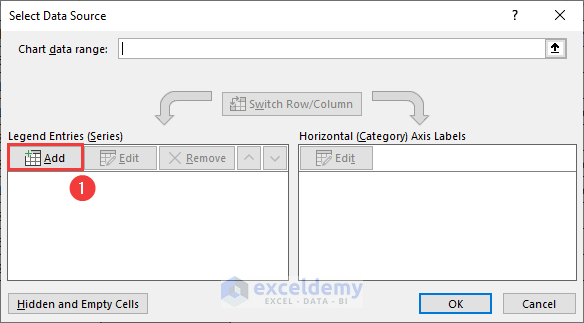
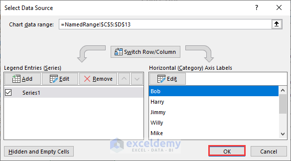
- A dialog box named Select Data Source appears.
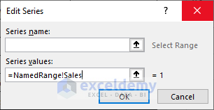
- Click on the Add command from the Legend Entries(Series) field.
- Enter =NamedRange!Sales in the Series values field.
- Hit the OK button.
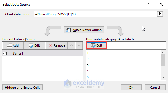
- Click on the Edit command from the Select Data Source dialog box.
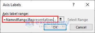
- Insert =NamedRange!Representatives in the Axis label range field.
- Hit OK.
- Load the Select Data Source dialog box by clicking on the OK button.
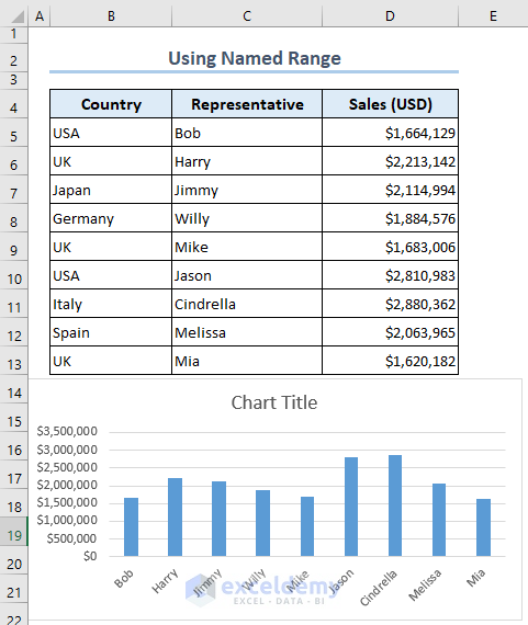
- Here’s the chart with all the data in the C4:C13 range.
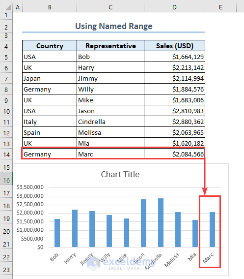
- Insert more information in the B14:D14 range.
Method 3 – Apply VBA Macro Tool to Develop Dynamic Charts
- Insert a blank chart. (go to Insert Column or Bar Chart and choose the 2-D Clustered Column chart type).
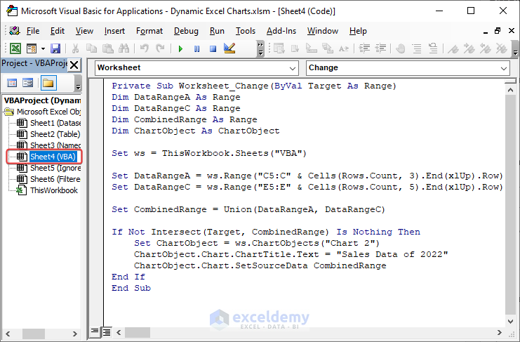
- Insert the following VBA code in the dedicated worksheet Module applying the VBA Worksheet Change event.
Private Sub Worksheet_Change(ByVal Target As Range) 'Developed by ExcelDemyDim DataRangeA As Range Dim DataRangeC As Range Dim CombinedRange As Range Dim ChartObject As ChartObject Set ws = ThisWorkbook.Sheets("VBA") Set DataRangeA = ws.Range("C5:C" & Cells(Rows.Count, 3).End(xlUp).Row) Set DataRangeC = ws.Range("E5:E" & Cells(Rows.Count, 5).End(xlUp).Row) Set CombinedRange = Union(DataRangeA, DataRangeC) If Not Intersect(Target, CombinedRange) Is Nothing Then Set ChartObject = ws.ChartObjects("Chart 2") ChartObject.Chart.ChartTitle.Text = "Sales Data of 2022" ChartObject.Chart.SetSourceData CombinedRange End If End Sub
Code Breakdown
- We create a Private Sub-Procedure in the worksheet module with a Change worksheet event. For every single change, it will run the code.
Private Sub Worksheet_Change(ByVal Target As Range)
[Your Code]
End Sub- Set ws as a worksheet (VBA) where the code will apply. Also, assigning the values of columns C and E in the DataRangeA and DataRangeC variables.
Dim ws As Worksheet
Dim DataRangeA As Range
Dim DataRangeC As Range
Set ws = ThisWorkbook.Sheets("VBA")
Set DataRangeA = ws.Range("C5:C" & Cells(Rows.Count, 3).End(xlUp).Row)
Set DataRangeC = ws.Range("E5:E" & Cells(Rows.Count, 5).End(xlUp).Row)- Using the VBA UNION function, we combine columns C and D. and assign the value in the CombinedRange variable.
Dim CombinedRange As Range
Set CombinedRange = Union(DataRangeA, DataRangeC)- The name of the blank chart is Chart 2. The IF statement dictates if Target and CombinedRange values don’t overlap then return outcome based on
ChartObject.Chart.SetSourceDataproperties and updates automatically. ChartObject.Chart.ChartTitle.Textproperties inserts the title of the chart.
Dim ChartObject As ChartObject
If Not Intersect(Target, CombinedRange) Is Nothing Then
Set ChartObject = ws.ChartObjects("Chart 2")
ChartObject.Chart.ChartTitle.Text = "Sales Data of 2022"
ChartObject.Chart.SetSourceData CombinedRange
End If
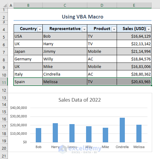
- We get the updated chart after adding the data for Melissa in the B11:E11 range.
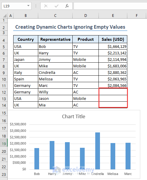
Create Dynamic Charts while Ignoring Empty Values in Excel
- Make a new Defined Name.
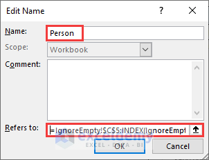
- Type Person in the Name field.
- Insert the following formula in the Edit Name dialog.
=IgnoreEmpty!$C$5:INDEX(IgnoreEmpty!$C$5:$C$11,COUNT(IgnoreEmpty!$C$5:$C$11))
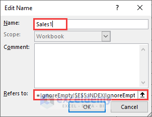
- Type Sales(1) in the Name field and use the formula as follows in the Edit Name dialog.
=IgnoreEmpty!$E$5:INDEX(IgnoreEmpty!$E$5:$E$14,COUNT(IgnoreEmpty!$E$5:$E$14))
- Get the Select Data Source dialog box by following the steps of the similar procedure of the Named Range approach.
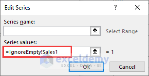
- Insert =IgnoreEmpty!Sales1 in the Series values field of the Edit Series dialog box.
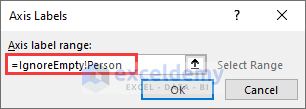
- Insert =IgnoreEmpty!Person in the Axis label range field of the Axis Labels dialog box.
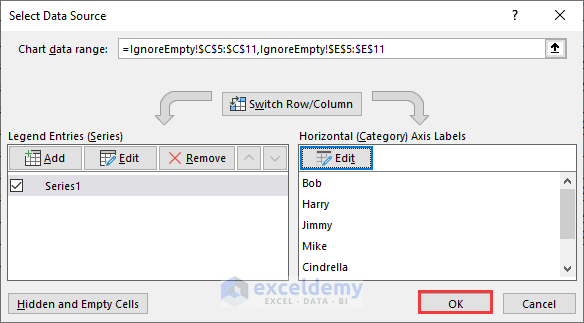
- Load the Select Data Source dialog box by hitting the OK button.
- We get the chart containing information on the representatives and ignore the blank cells.
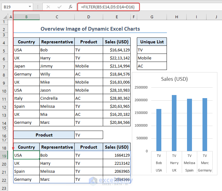
How to Create Filtered Dynamic Charts in Excel
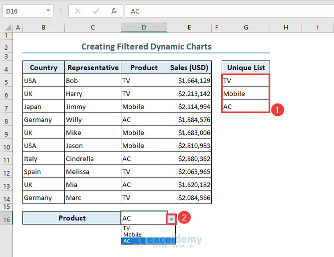
- Create a unique list in the G5:G7 range by inserting the following formula containing the UNIQUE function in the G5 cell:
=UNIQUE(D5:D14)
- Make a drop-down list in the D16 cell by using the Data Validation tool.
- Use the following formula containing the FILTER function in the B19 cell to obtain filtered data based on the selection of the drop-down list.
=FILTER(B5:E14,D5:D14=D16)
- Create a chart by clicking on the Insert Column or Bar Chart command that we mentioned earlier.
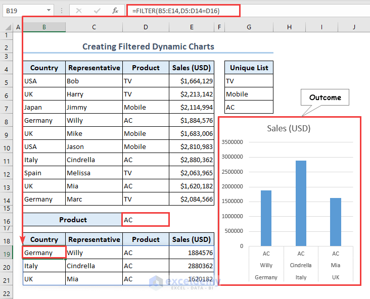
- By selecting TV from the drop-down list of the D16 cell, we get filtered results in the B19:E22 range as well as a Clustered Column chart.
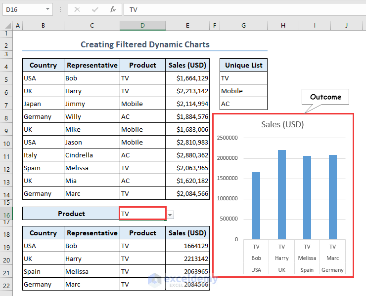
Note: You will not get the FILTER function in any other versions without Microsoft Office 365, Excel 2019, and 2021.
Frequently Asked Questions
What does a dynamic chart do in Excel?
Dynamic charts in Excel update automatically once new rows containing data are added or removal of rows takes place.
What are dynamic charts vs. static charts in Excel?
Dynamic charts update automatically with the inclusion or exclusion of data from the selected range. On the other hand, static charts don’t update by employing new rows in the dataset.
What is keyboard shortcut to create Excel charts?
By selecting the dataset and pressing the Alt + F1 keys, you can create Excel charts.
Dynamic Excel Charts: Knowledge Hub
<< Go Back to Excel Charts | Learn Excel
Get FREE Advanced Excel Exercises with Solutions!
