When you are working with a dataset that needs to plot on a chart, you will try to create dynamic Excel charts with a drop-down list. A dynamic chart can automatically change its shape in case you alter any data. There is also a process which you can add a drop-down list through. A drop-down list can help you to focus on a certain product or country and its dynamic chart. This article will mainly focus on how to create dynamic Excel charts with a drop-down list in an effective way.
To create dynamic Excel charts with a drop-down list, we have found three different methods through which you can have a complete overview of this topic. All of these methods are fairly easy to understand. Here, we basically utilize an Excel table, a data validation process, and finally, utilize a combo box to create a drop-down list. After that, we create a dynamic chart.
1. Using Table to Create Dynamic Excel Charts with Drop-Down List
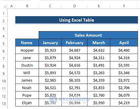
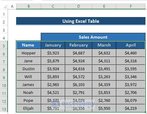
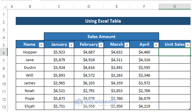
Our first method is basically the use of an Excel table. At first, we create a drop-down list by using data validation. After that, we create an Excel table using the drop-down list and finally plot it on an Excel chart. To do this, we take a dataset that includes several months’ sales amount of some salesmen.
To understand the method properly, you need to follow the steps.
Steps
- At first, we need to create the drop-down list using the data validation.
- Select cell J4.
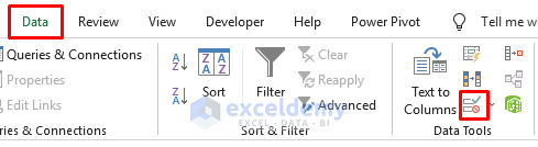
- Then, go to the Data tab in the ribbon.
- From the Data Tools group, select the Data Validation option.
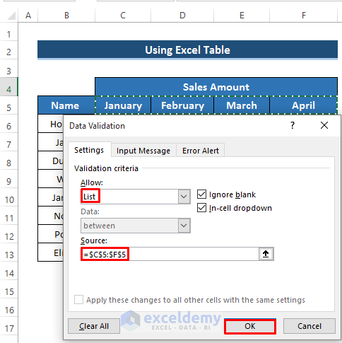
- After that, the Data Validation dialog box will appear.
- Then, in the Validation Criteria section, select the List option from the Allow drop-down option.
- In the Source section, select the range of cells C5 to F5.
- Finally, click on OK.
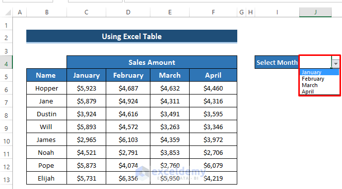
- It will create a drop-down option in cell J4.
- As we gave the months as the Source, so, we can select any months from that drop-down option.
- Now, we need to convert the dataset into a table.
- At first, select the range of cells B5 to F13.
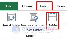
- Then, go to the Insert tab in the ribbon.
- From the Tables group, select the Table option.
- Then, the Create Table dialog box will appear.
- Click on OK to create the required table.

- Then, you’ll get the required table. See the screenshot.
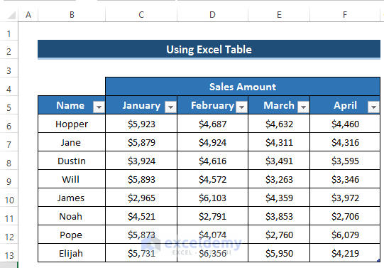
- Then, create another column beside April.
- The New column will be known as ‘Unit Sales’.
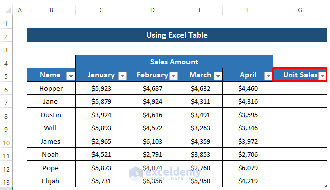
- Then, select cell G6.
- Write down the following formula in the formula box using the SUMIF function.
=SUMIF($C$5:$F$5,$J$4,$C6:$F6)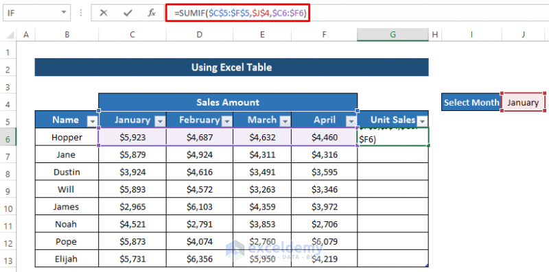
🔎 Breakdown of the Formula
SUMIF($C$5:$F$5,$J$4,$C6:$F6): The SUMIF function returns the sum of the range of cells that meet certain criteria. Here, the first part of the SUMIF function is the range of cells where the criteria will be applied. The second part is the criteria. The last part is the range containing values to sum. Here, our criteria is a month for example January. This criterion will be applied in the first range of cells. Then, go to the last range to find out the values to sum. Finally, it returns the value of January.
- Press Enter to apply the formula.
- It will automatically fill the whole table. See the screenshot.
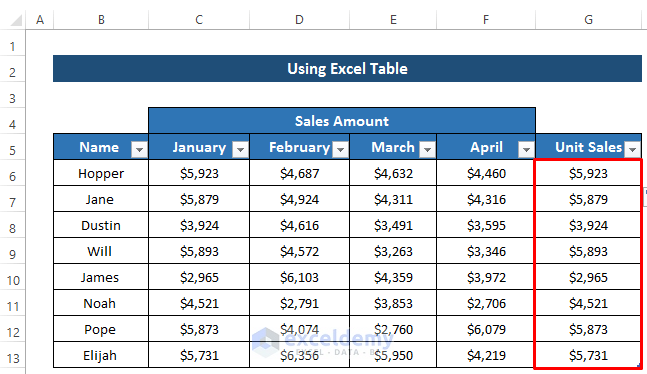
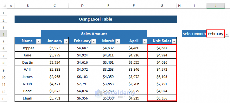
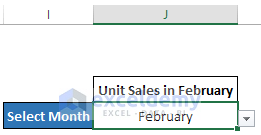
- Then, if you change the month in the drop-down option, it will automatically change it in the Unit Sales column.
- After that, we want to create a dynamic chart title that changes with the drop-down option.
- To do this, select cell J3.
- Write down the following in that cell to create a link with the drop-down option.
="Unit Sales in"&" "&J4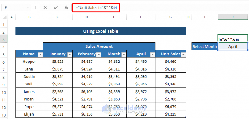
- Press Enter to apply it.
- Then, when you alter the drop-down option, it will automatically change it in cell J3.
- Then, we need to create the dynamic chart.
- To do this, go to the Insert tab in the ribbon.
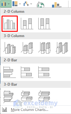
- From the Charts group, select the Column chart drop-down option.
- Here, you’ll get several column chart options.
- Select the first 2-D column chart option.
- It will create a blank chart.
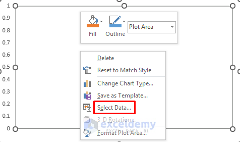
- Then, right-click on it to open the Context Menu dialog box.
- Select the Select Data option.
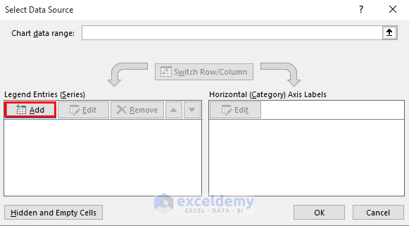
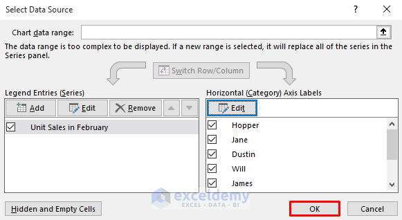
- It will open up the Select Data Source dialog box.
- From the Legend Entries(Series) section, click on Add.
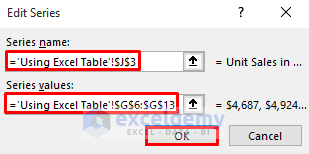
- Then, in the Edit Series box, set the Series name and Series values.
- After that, click on OK.
- Then, in the Horizontal Axis Labels section, click on Edit.
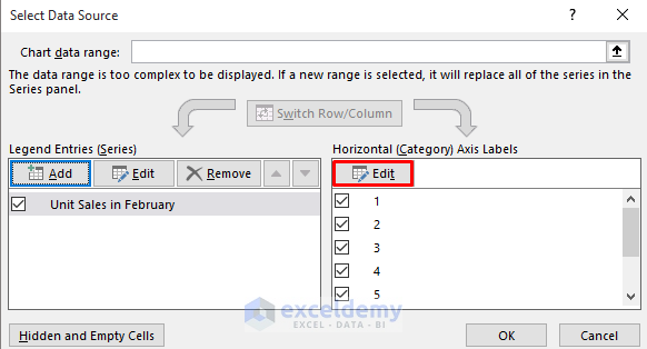
- Select the range of cells B6 to B13 as horizontal axis labels.
- Then, click on OK.
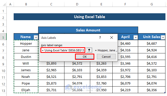
- Finally, click on OK in the Select Data Source dialog box to represent this in the chart.
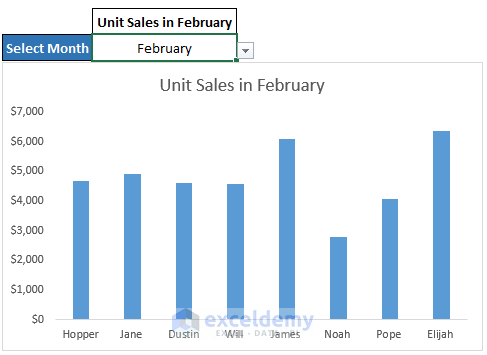
- It will give us the following results. See the screenshot.
- To change the Chart Style, click on the Brush icon on the right side of the chart.
- Then, select any of the chart styles.
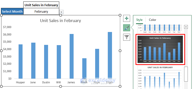
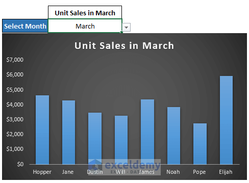
- Finally, we’ll get our required dynamic Excel chart with a drop-down option.
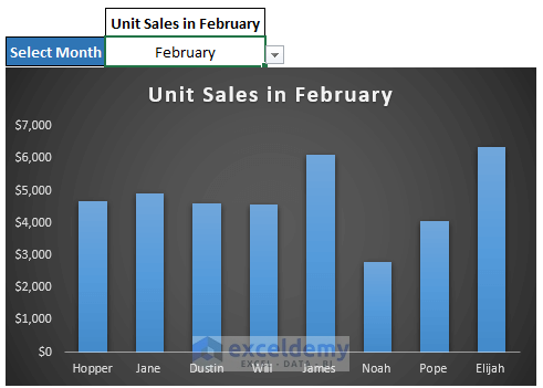
- Then, if you change the month from the drop-down option, it will change the whole chart. See the screenshot.
Read More: How to Create Dynamic Charts in Excel Using Data Filters
2. Applying Data Validation for Creating Dynamic Charts with Drop-Down List
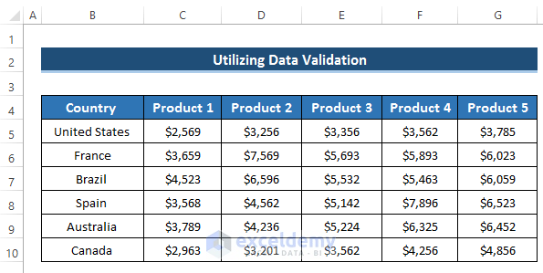
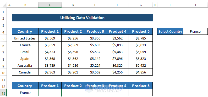
Our second method is based on using data validation. Here, we basically create a drop-down option using the data validation option. After that, we use the INDEX and MATCH functions to create a dynamic chart. To show this method, we take a dataset that includes several countries and their several products sales amount.
To use the methods carefully, you need to follow the steps carefully.
Steps
- At first, we need to create the drop-down list using the data validation.
- Select cell J4.
- Then, go to the Data tab in the ribbon.
- From the Data Tools group, select the Data Validation option.

- After that, the Data Validation dialog box will appear.
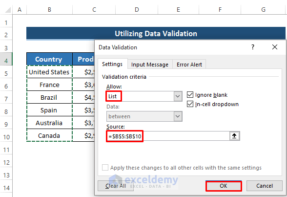
- Then, in the Validation Criteria section, select the List option from the Allow drop-down option.
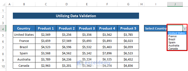
- In the Source section, select the range of cells B5 to B10.
- Finally, click on OK.
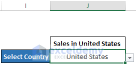
- It will create a drop-down option in cell J4.
- As we gave the countries as the Source, so, we can select any country from that drop-down option.
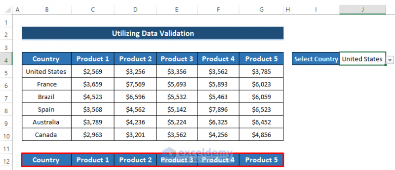
- Then, we need to turn our focus on creating a dynamic Excel chart.
- At first, we create some row headers similar to our dataset.
- Then, in cell B13, write down the following formula to link with the drop-down option.
=J4- Press Enter to apply this.
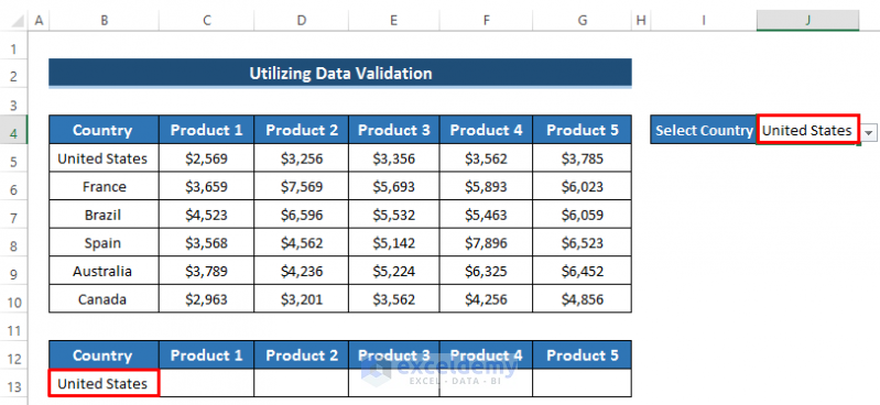
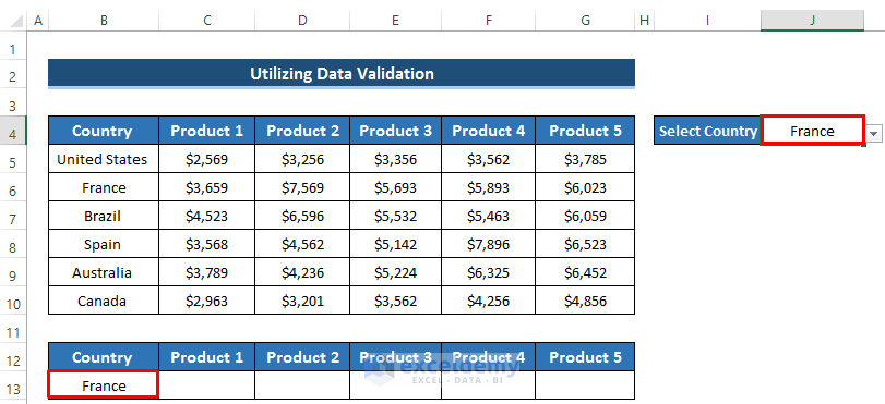
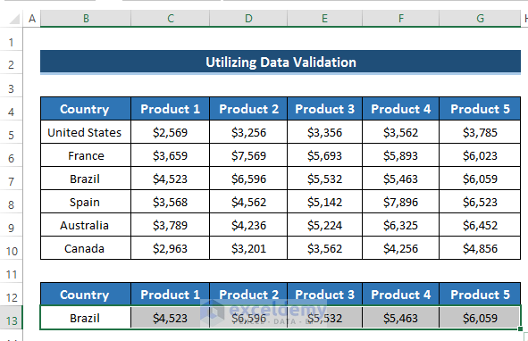
- Then, if you change the drop-down option from the United States to France, it will automatically change in cell B13.
- Then, select cell C13.
- Write down the following formula in the formula box.
=INDEX($C$5:$G$10,MATCH($J$4,$B$5:$B$10,0),MATCH(C4,$C$4:$G$4,0))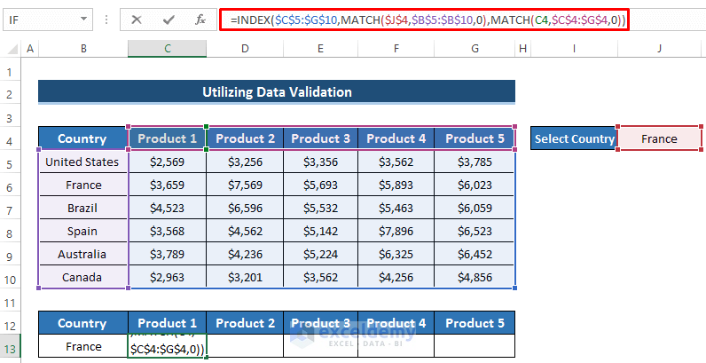
🔎 Breakdown of the Formula
⇒ MATCH($J$4,$B$5:$B$10,0): At first, we set a lookup value. Here, the country name is the lookup value which is created by the drop-down option. Then, set the lookup array from cell B5 to B10, and finally, we set an exact match of these lookup values. So, when we set the United States in the drop-down option, the MATCH function will look up the country in the given lookup array.
⇒ MATCH(C4,$C$4:$G$4,0)): In this function, we set product 1 as the lookup value. the MATCH function will look up product 1 in the given lookup array and find it as an exact match.
⇒ INDEX($C$5:$G$10,MATCH($J$4,$B$5:$B$10,0),MATCH(C4,$C$4:$G$4,0)): Finally, the INDEX function will return the value within the given range of cells.
- Press Enter to apply the formula.
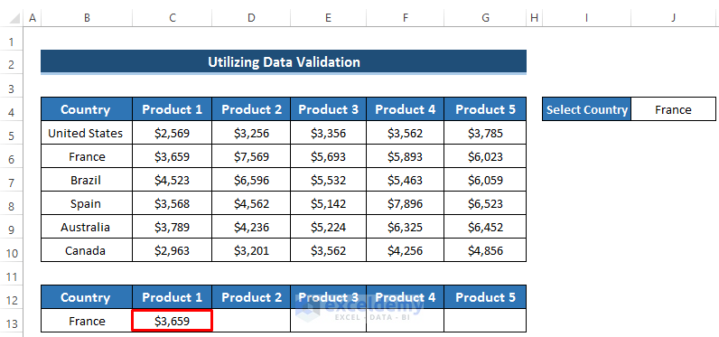
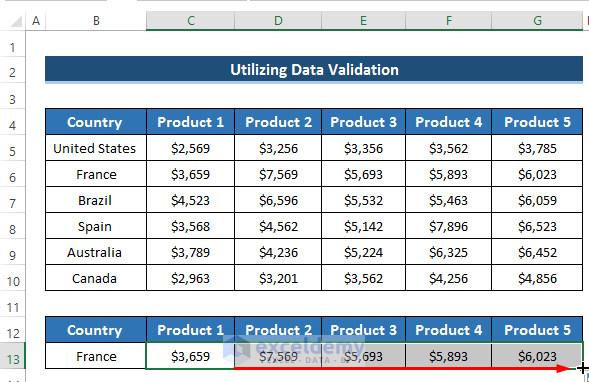
- Then, drag the Fill Handle icon up to cell G13.
- After that, we want to create a dynamic chart title that changes with the drop-down option.
- To do this, select cell J3.
- Write down the following in that cell to create a link with the drop-down option.
="Sales in"&" "&J4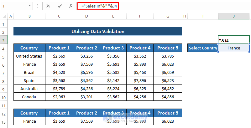
- Press Enter to apply it.
- Then, when you alter the drop-down option, it will automatically change it in cell J3.
- To create a dynamic Excel chart, select the range of cells B13 to G13.
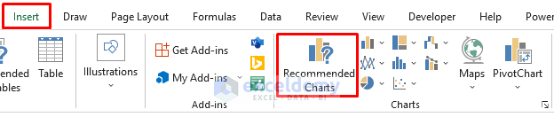
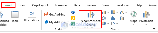
- Then, go to the Insert tab in the ribbon.
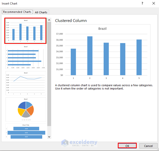
- From the Charts group, select Recommended Charts option.
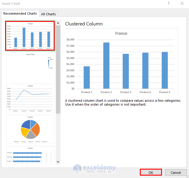
- An Insert Chart dialog box will appear.
- From there, select the Clustered Column chart.
- Then, click on OK.
- There we have our dynamic charts with a drop-down option.
- But, we need to modify the chart to have a better look.
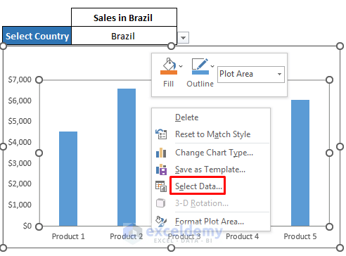
- Right-click on the chart to open the Context Menu.
- Then, from there, select the Select Data option.
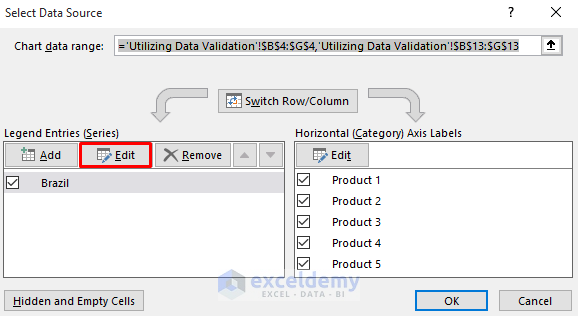
- Then, the Select Data Source dialog box will occur.
- From the Legend Entries (Series) section, select Edit.
- Then, change the Series name and set the cell J3 as reference.
- After that, click on OK.
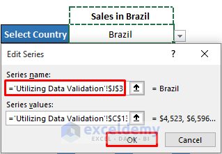
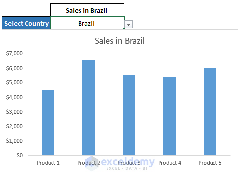
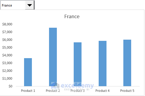
- Finally, click on OK in the Select Data Source dialog box.
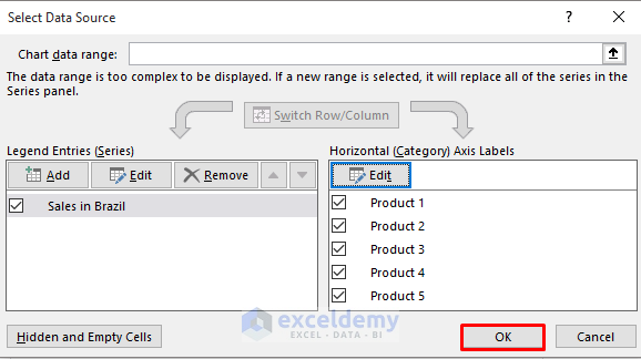
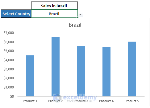
- It will give us the following results. See the screenshot.
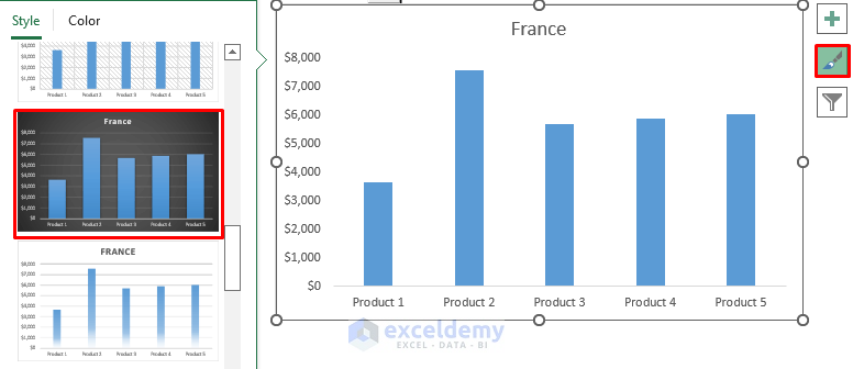
- Then, if you want to change the Chart Style of your dynamic chart, you need to click on the Brush icon on the right side of the chart.
- Select your preferred chart style.
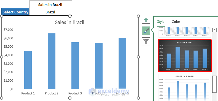
- It will give us the following results.
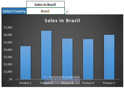
- Now, if you change the country from the drop-down option, it will change the chart and set it for that specific country.
Read More: How to Create Dynamic Chart with Multiple Series in Excel
3. Inserting INDEX Function to Create Dynamic Excel Charts with Drop-Down List
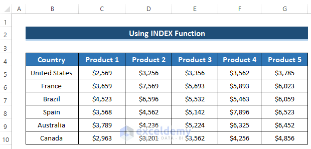
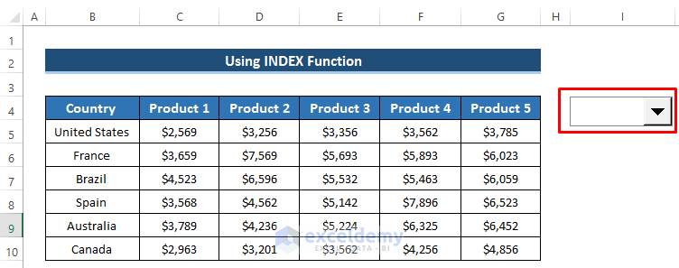
In our third Method, We will utilize the INDEX function to create a dynamic Excel chart with a drop-down list. Here, we basically create a dynamic chart in Excel where we can see the preview of several product sales amounts in the corresponding countries. To show the process completely, we take a dataset of several countries and five different product sales amounts.
Follow the steps carefully.
Steps
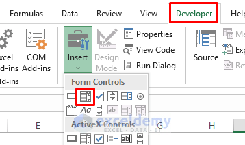
- At first, go to the Developer tab in the ribbon.
- From the Controls group, select the Insert drop-down option.
- Then, from the Form Controls section, select Combo Box.
- After that, in any cell draw a box. It will shape up like the following one. See the screenshot.
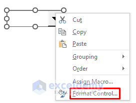
- Then, to modify it, right-click on it.
- A Context Menu will appear. From there, select the Format Control option.
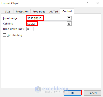
- After that, the Format Object dialog box will appear.
- In the Input range section, select the countries range because we want to plot a chart for a specific country.
- Then, select a cell link. It will change along with the combo box drop-down option.
- Finally, click on OK.
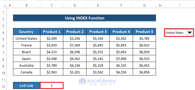
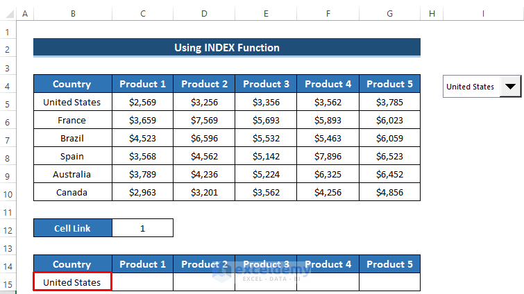
- Now, click on the drop-down option of the combo box.
- You will find out all the countries’ names from your dataset.
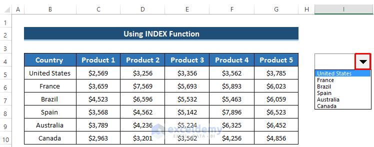
- Select any country and see the cell link will also change.
- Here, our first country in the United States. So, if you select it, the cell link will show 1 as the first country.
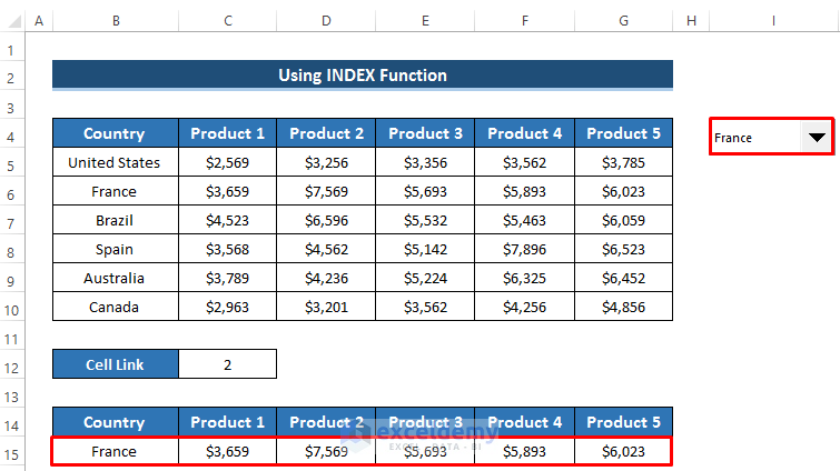
- If you select France from the drop-down option, the Cell link will show 2.
- After that, we want to utilize this cell link and the INDEX function to create a dynamic Excel chart.
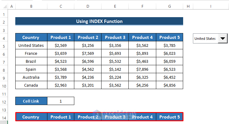
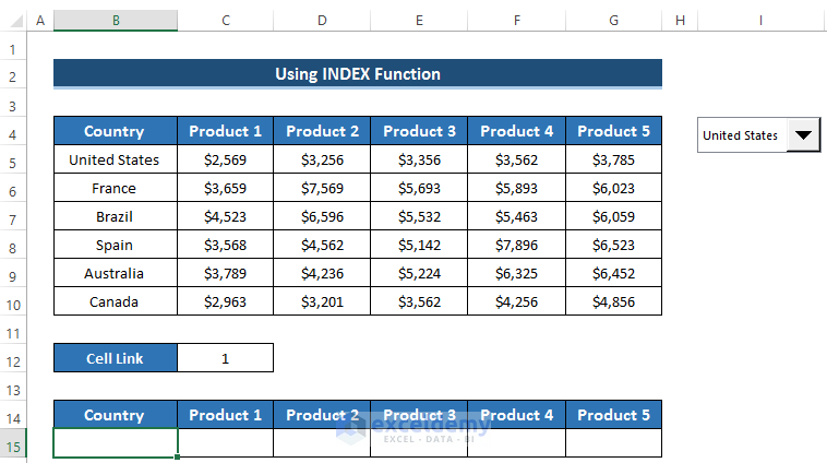
- First, create some headers for the dynamic chart.
- Then, select cell B15.
- Write down the following formula in the formula box.
=INDEX(B5:B10,$C$12)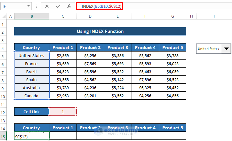
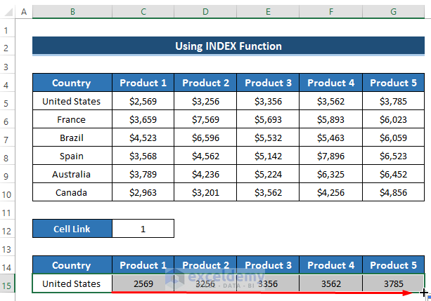
- Press Enter to apply the formula.
- Then, drag the FIll Handle icon right up to cell G15.
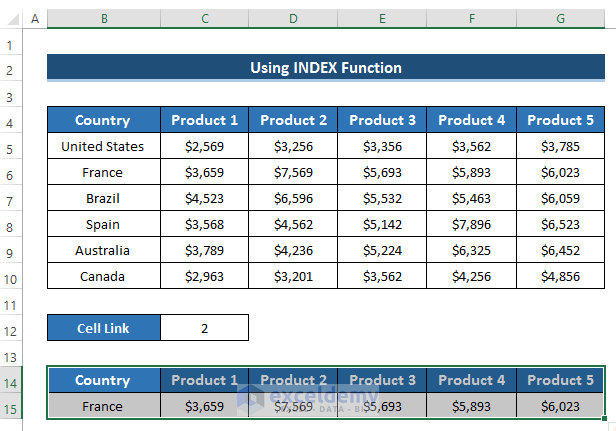
- Now, change the country from the drop-down option and select France.
- Then, look at the dynamic table All the values of that table change and shift to France and its corresponding products sales amount.
- Select the range of cells B14 to G15.
- Then, go to the Insert tab in the ribbon.
- From the Charts group, select Recommended Charts option.
- After that, the Insert Charts dialog box will appear.
- From there, select the Clustered Column chart.
- Finally, click on OK.
- As a result, we get a dynamic chart.
- Then, to change the Chart Style, select the brush icon.
- After that, select your preferred style.
- Finally, we get the following result. See the screenshot.
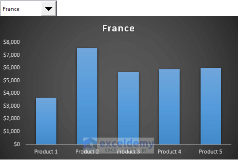
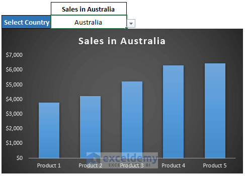
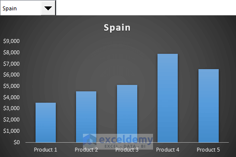
- As it is a dynamic chart, you can alter the drop-down option and select any country.
- The chart will represent that country.
- Here, we select Spain from the drop-down option. See the result in the following screenshot.
Read More: How to Create Chart with Dynamic Date Range in Excel
Things to Remember
- You can create drop-down options by using a combo box or data validation. Both of them are effective but for better results, you may consider the data validation process.
- As we use a combination of INDEX and MATCH functions, you need to use them carefully. Otherwise, you’ll get errors.
Download Practice Workbook
Conclusion
We have shown three different methods to create dynamic Excel charts with a drop-down list. All of these methods are really effective to use. In every method, we try to create a drop-down list using a combo box or data validation. After that, we created the dynamic charts. All of these methods give you some precise solutions which will be very helpful for your further purpose. If you have any more questions, feel free to ask in the comment box. Don’t forget to visit our ExcelDemy page.
Related Articles
- How to Make Dynamic Charts in Excel
- How to Create Min Max and Average Chart in Excel
- Create a Dynamic Chart Range in Excel
- How to Dynamically Change Excel Chart Data
- How to Create a Dynamic Chart in Excel Using VBA
<< Go Back to Dynamic Excel Charts | Excel Charts | Learn Excel
Get FREE Advanced Excel Exercises with Solutions!
