Latest Posts From Durjoy Paul
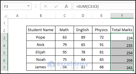
Dataset Overview To illustrate these methods, we'll use a dataset containing the report cards of some students. This dataset includes marks for three ...

Method 1 – Importing Data From PDF to Excel Steps: Open an Excel file. Go to the Data tab on the Ribbon. Select the Get Data option from the Get ...
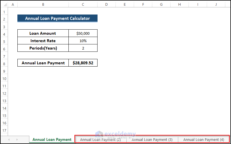
Open your Excel workbook. Locate the sheet you want to duplicate in the bottom tab bar. Right-click on the sheet tab to bring up the Context Menu. ...

Step 1 - Convert Excel to CSV File Open the Excel file which you want to convert into a CSV file. Place a dataset that contains some names and their ...

Method 1 - Using Conventional Formula to Calculate 3-Year CAGR Steps To calculate the CAGR in Excel, select cell C10. Write down the following ...
Method 1 - Using Text to Columns from the Data Tab Steps: Select cell B5. Enter the name ‘Elijah Williams’. Press Alt+Enter to create ...
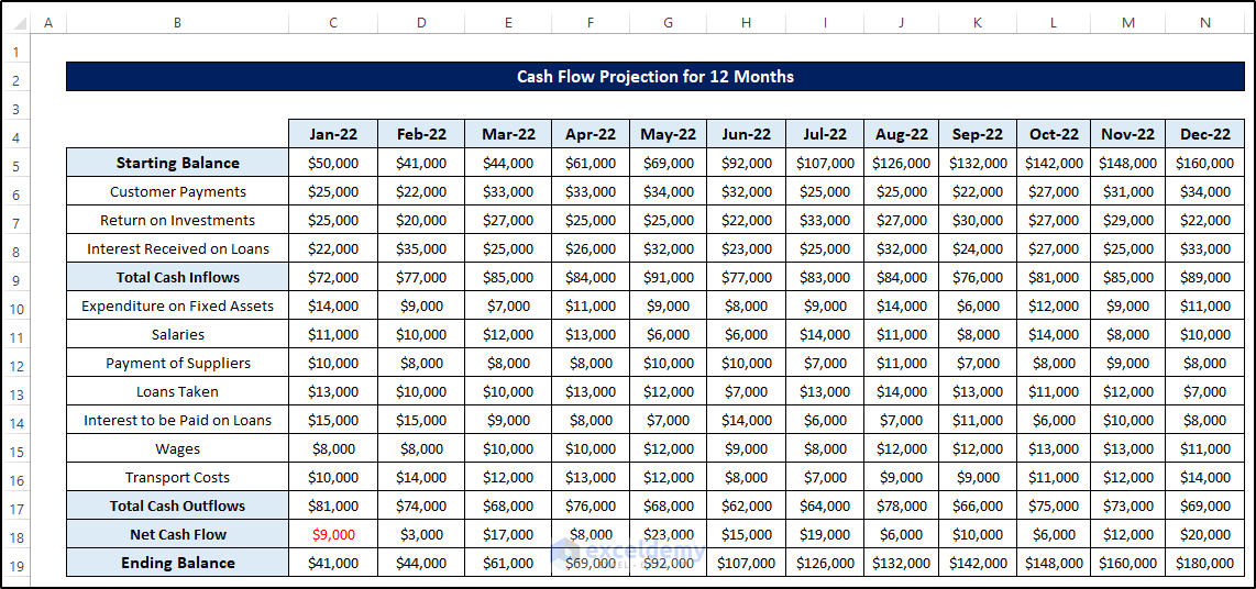
Overview A cash flow model is a financial statement that describes the inflows and outflows of cash over a certain period for a specific organization or ...
What Is Cap Percentage? Cap percentage can be defined as a percentage limit in which your dataset percentage will be contained. For example, you want to ...

Annual Loan Payment Overview The annual loan payment is the total principal amount and interest amount that is paid in a year. To calculate it, you need to ...
Method 1 - Calculate EMI Use the PMT function to calculate EMI and then produce the EMI calculator, taking some values. With these values, calculate the EMI, ...

Sometimes, you need to calculate the average of a big group. Calculating the average manually is a time-consuming process. That’s why we can take the ...

When you enter any number in the Excel worksheet cell, you will see the number will align on the right side of the cell as a default. This is a normal ...
Method 1 - Finding Average Marks of Each Exam Steps We would like to find the average, excluding the absent text. Select cell C13. Write down the ...

How to Create a 3D Reference in Excel The workbook contains students' marks in different subjects and in different exams. Create a dataset for ...

This article will demonstrate how to add up and down buttons to increase and decrease cell value in Excel. How to Add Up and Down Buttons in Excel: ...
- 1
- 2
- 3
- …
- 8
- Next Page »
See Our Reviews at


Hi Niki,
To find out the price, you need to calculate the product of unit and unit quantity. Your sheet 1 denotes the unit of rate 1, rate 2, rate 3, and rate 4. The unit quantity will be found in sheet 2. So, in that case, you can apply the VLOOKUP formula to get the specific unit and unit quantity. You can use the following formula to calculate.
=VLOOKUP(J8,$B$7:$C$12,2,FALSE)*VLOOKUP(J8,Sheet1!$B$4:$C$8,2,FALSE)
=VLOOKUP(J8,$B$7:$C$12,2,FALSE):
First, you need to define the value you are looking for. Here, J8 refers to the lookup value. After that, define the table array where you think the required answer can remain. Then, define the column number of the expected result. Finally, use false to get the exact match. Then, we have to multiply the result of the first VLOOKUP by the result of the second VLOOKUP.
VLOOKUP(J8,Sheet1!$B$4:$C$8,2,FALSE):
As we put the unit in sheet 1, we have to look up the rate 1 unit by utilizing the VLOOKUP function. First, define rate 1 as the lookup value. Then, set the table array in sheet 1. After that, define the column number of the expected result. Finally, use false to get the exact match.
The product of these two values will give the price of rate 1. Do the same procedure for other cases.
Do you get your preferred answer? check on it. Otherwise, give us a more accurate question. We are always ready to help you.
Thank you.
Hello Anton,
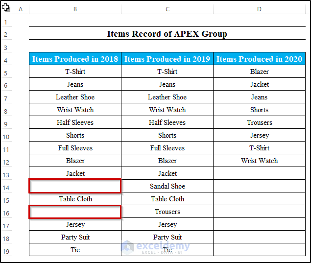
First of all, you have to create three columns including items produced in 2018. Here, we need to paste the same value as items produced in 2019. Just one or two blanks in there.
Then, take a new cell and write down the following formula.
=IF(COUNTIF(D5:D12,B5:C19)>0,B5:C19,””)
Here, the range becomes (D5:D12 as the column of items produced in 2020 changes. Then, the criterion becomes B5:C19. Here, it follows if the condition match for both cells then it will return the value. Otherwise, it returns blank. After that, press Ctrl+Shift+Enter as it is an array formula.
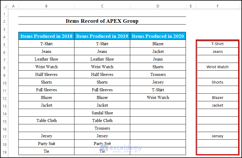
Here, you can see, that the product Trousers is available in 2019 and 2020. but, we give criteria for products in 2018 and 2019. As they don’t find trousers in 2018, that’s why you won’t get them in the result. So, you will get the products that are available in both 2018 and 2019.
Hello BOMBSHELLSHOCK, first, you need to convert your dataset into Excel table format. To do that, you have to select your whole dataset and go to the Insert tab on the ribbon. After that, select Table from the Tables group. As a result, it will convert your dataset into a table. Then, you can write something in the last row and column and press Enter. As a result, Excel will insert new rows and columns into your Excel table. So, to perform the whole process, you must convert your dataset into a table. Mind it.
If you face any more problems, you can share them with us. We are happy to deal with it and provide you with a proper solution.
Hello Tomas,
You can store these non-object events in a personal file module. The solution is applicable to any module. First, you need to define the time value perfectly. To do that, you may use the following code.
Application.OnTime TimeValue(“11:48:00 am”), “DisplayAlarm”
If you set the time value properly, then there will be no problem in any module. Hope you get your required solution.
Hello Nathan,
first of all, if you want to use sum color function, you can use the following code.
Function SumByCol(SumRange As Range, SumColor As Range)
Dim SumColValue As Integer
Dim TotSum As Long
SumColValue = SumColor.Interior.ColorIndex
Set pCell = SumRange
For Each pCell In SumRange
If pCell.Interior.ColorIndex = SumColValue Then
TotSum = TotSum + pCell.Value
End If
Next pCell
SumByCol = TotSum
End Function
Then, close the VBA code and select any cell where you want to put the sum value. After that, write the following formula
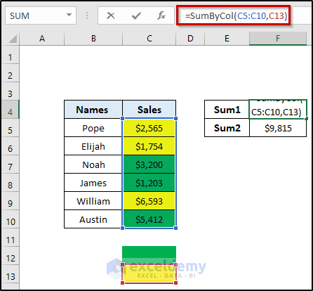
=SumByCol(C5:C10,C13)
Where the range of cells C5 to C10 defines the range. C13 defines the color. You need to show only color in one cell. From where you can take the reference. Here, C13 denotes that color reference. So, when you want to change the color, you have to change the color reference also.
Hello Helen,
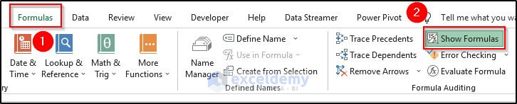
You can do it without using the find and replace command. To do this follow the steps carefully.
1. First, go to the Formula tab on the ribbon.
2. Then, Select Show Formulas from the Formula Auditing section.
3. As a result, it will show you the formulas that you use in the workbook.
4. Now, copy the formulas and paste them into a notepad.
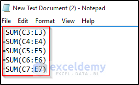
5. Then, press Ctrl+A to select all and after that, press Ctrl+C to copy.
6. In a new workbook, paste it by pressing Ctrl +V. As a consequence, you will see the formulas are copied accurately without a reference workbook.
Hello Mark,
We have sent you a mail. Can you see it and give us a response?
Hello Craig,
We are not dealing with SharePoint at this moment. So, I can’t give you a proper solution to this problem. In the future, if we work with SharePoint, we will get back to you and provide you with a useful solution.
Thanks.
Hello Jorge,
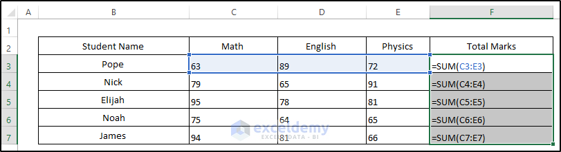
This is an array formula. It must be completed by pressing Ctrl+Shift+Enter. Otherwise, it won’t work. For a normal formula, we press only Enter. But for an array, you have to press Ctrl+Shift+Enter. I hope you get your solution. If you find any more problems, feel free to ask in the comment box. We are always here to help you.
Hello Laura,
I hope you are doing well. If you want to use a VBA code that can only paste values instead of a straight paste, you may use the following one.
Sub Paste_Row_Values()
a = Worksheets(“Dataset2”).Cells(Rows.Count, 1).End(xlUp).Row
For i = 2 To a
If Worksheets(“Dataset2”).Cells(i, 4).Value = “CLAIMS” Then
Worksheets(“Dataset2”).Rows(i).Copy
Worksheets(“CLAIMS”).Activate
b = Worksheets(“CLAIMS”).Cells(Rows.Count, 1).End(xlUp).Row
Worksheets(“CLAIMS”).Cells(b + 1, 1).Select
ActiveCell.PasteSpecial Paste:=xlPasteValues
Worksheets(“Dataset2”).Activate
End If
Next
Application.CutCopyMode = False
ThisWorkbook.Worksheets(“Dataset2”).Cells(1, 1).Select
End Sub
I think you get your required solution. By using this code, you can paste the row values without any format. If you have any further queries, feel free to connect us.
Hello Kane,
You need to put the picture in one cell. Just resize it and put the image in a single cell then apply the sorting. I think you will get your desired result.
1. First, change the row height of the cell to adjust the image in the cell or resize it to adjust it in a single cell.
2. Then, select the range of cells. Go to the Data tab and select your preferred sorting.
3. Finally, you will see the image is also changing its place while sorting.
Hello rick, Thanks for your valuable feedback.
Hello Mark SIMONS and GVG,
Can you please share your Excel dataset with us? Then, we will try our best to provide you with the required solution.
Hello Thanks,
In the first 4 paragraphs, we use =VLOOKUP(D14,B4:F12,5,FALSE) this formula. Here, we define the range of cells. So, when we define column number as 5, Excel will count from column B as the first column.
Whereas, =VLOOKUP($C5,$H$5:$J$9,COLUMN()-3,0) in this equation, we use Column() function. This function will count the column number from column A. So, when you have COLUMN()-3 and are in column E, it will be 5-3= 2.
So, I hope you understand it clearly. If you have further queries, feel free to ask in the comment box.
Hello Roger,
Can you please share your Excel dataset with us? We will try our best to solve your problem. Because in our Excel 365, the conditional formatting works perfectly for absolute and relative cell references in both cases.
Hello UGEN,
First, select the range of cells including the column with merged cells. Then, press Alt+;(Semicolon) which will select your visible cells only. After that, press Ctrl + C to copy. Finally, apply Ctrl+V to paste the range of cells into your desired position. I hope this will solve your problem. If you have any more questions, feel free to contact us. We will try our best to solve the problem.
Hello Tawfik,
Can you please share your Excel file with us? We will try our best to solve your problem.
Hello Swaroop,
can you please share your Excel file and explain the question clearly?
Because we didn’t sort our first two rows in this example also.
Hello, Can you please email us your Excel dataset with the problem?
We will try our best to give you a proper solution.
Hello Chris, in option one, you need to insert the VBA code first. After that, you can apply the ColorFunction. Otherwise, you will face difficulties.
If you don’t get the solution yet, you can send your worksheet. We will take a look closely and find the required solution.
Hi Henrik, to highlight rows in Excel, you need to apply VBA code in that certain worksheet like this article. Otherwise, you need to run the code every time when you go to the next row and highlight it. This is a major disadvantage of this method. If you need to apply in all the worksheets, then you need to utilize the following code.
Sub Highlights_Active_Row()
Static xRow
If xRow <> “” Then
With Rows(xRow).Interior
.ColorIndex = xlNone
End With
End If
Active_Row = Selection.Row
xRow = Active_Row
With Rows(Active_Row).Interior
.ColorIndex = 7
.Pattern = xlSolid
End With
End Sub
Note: Remember every time you go to the next row, you have to run the code every single time.
Hi Amber, You can’t undo anything after applying the VBA code. This is one of the drawbacks of Excel.
Hello Brow, yes you are right. It should be Row(A1) = HighlightActiveRow
Hey Luna, did you solve the problem using the VBA code? If you face further problems, feel free to share them in the comment box. We are eager to help you to get the desired result.
Hey Max, try the following VBA code
Sub Changing_Date_Format_Using_Condition()
Dim i As Integer
i = InputBox(“Enter a Number”)
If i = 2 Then
Range(“A1”).NumberFormat = “mm/dd/yyyy”
ElseIf i = 10 Then
Range(“A2”).NumberFormat = “dddd-dd-mmm-yy”
Else
Range(“A3”).NumberFormat = “mmm-yy”
End If
End Sub
Is this your required solution? If not then explain more about it. We will help you to get the result.
Hey Stacy, You can read the following article to get just the date to display in the linked cell
https://www.exceldemy.com/insert-drop-down-calendar-in-excel/#Step_4_Link_Drop_Down_Calendar_to_a_Cell_in_Excel
Otherwise, you can go to the developer tab on the ribbon. Then, select Add-ins from the Add-ins group. In that Add-ins, add Mini Calendar and Date Picker. From there, you can add only the date in the linked cell.
Try this solution, I think you will get your desired result. If you have more problems inform us.
⇒OFFSET($B$2,ROUNDUP(ROWS($1:1)/3,0)-1,MOD(ROWS($1:1)-1,3)) : In the OFFSET formula, you need to put the cell reference, rows and cols number.
⇒OFFSET($B$2………): Here $B$2 is the cell reference of the OFFSET function.
⇒OFFSET($B$2, ROUNDUP(ROWS($1:1)/3,0)-1……): Here, the ROUNDUP function gives the specific number of rows down. ROWS function provides the number of rows in a given array. Here, the cell reference is $1:1. So, the Rows function returns 1. As we have three rows in our dataset. So, divide the return value of the Rows function by 3. It will return 0.333. Then, the ROUNDUP value will round the number into the nearest whole number. The whole number of 0.333 is 1. After that, subtract 1 from it. So, the final value is 0 which is the required rows down.
⇒OFFSET($B$2,ROUNDUP(ROWS($1:1)/3,0)-1,MOD(ROWS($1:1)-1,3)): To extract the columns right, we utilize the MOD function. It gives a reminder after a number is divided by the divisor. First, the Rows function provides the number of rows from the given array. Here, it returns 1. Then, subtract 1 from the return value. Then, divide the value by the total number of columns. The MOD function will return the reminder. Here, it returns 0.
So, for cell reference $B$2 and rows 0 down and cols 0 right, it returns Arif as our answer. Do the same for other cases.
Try this solution I think you will get your desired result. If you face any more problems, inform us.
To extract color information of conditional formatting cells, you need to follow the steps
1. First, use the conditional formattings in your dataset.
2. Then, click on the Dialog Box Launcher (Small tilted arrow beside Clipboard) from the Clipboard group.
3. After that, click on Clear All from there.
4. Copy the conditionally formatted range.
5. Now, select a new cell where you want to paste your conditional formatting range color only.
6. After that, click on Paste All from the Clipboard group.
7. Now, remove the numbers and only remains the conditional formatting colors.
8. Now, use =Background or =getLeftColor or =getRightColor just like this article, you will get your desired color information.
Try this solution I think you will get your desired result. If you face any more problems, inform us.