Method 1 – Using Conventional Formula to Calculate 3-Year CAGR
Steps
- To calculate the CAGR in Excel, select cell C10.
- Write down the following formula.
=(C8/C5)^(1/3)-1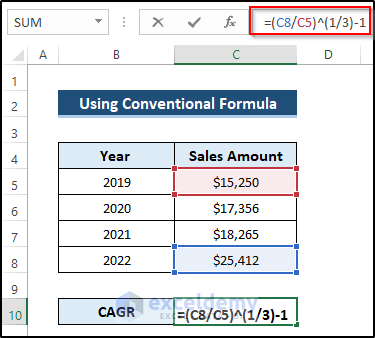
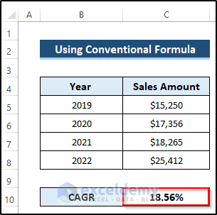
- Press Enter to apply the formula.
Method 2 – Applying the RATE Function
Steps
- To calculate the CAGR in Excel, select cell C10.
- Write down the following formula.
=RATE(ROW(C8)-ROW(C5),,-C5,C8)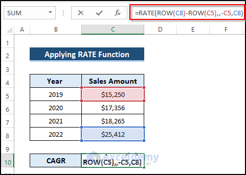
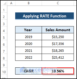
- Press Enter to apply the formula.
Breakdown of the Formula
RATE(ROW(C8)-ROW(C5),,-C5,C8): The ROW function returns the row number of the C8 and C5 cells. The RATE function returns the interest rate per period of a loan or investment. 3 is the upper argument that represents the number of periods; the pmt argument is left blank; the C5 cell refers to the Pv argument, which indicates the Initial Value of $15250, and the C8 cell is the fv argument that points to the Final Value of $25412.
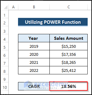
Methods 3 – Utilizing the POWER Function to Calculate 3-Year CAGR
Steps
- To calculate the CAGR in Excel, select cell C10.
- Write down the following formula.
=POWER(C8/C5,1/3)-1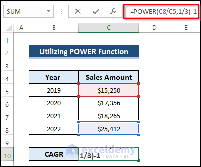
- Press Enter to apply the formula.
Breakdown of the Formula
POWER(C8/C5,1/3)-1: The function returns the result of a number raised to a power. C8/C5 is the number argument that refers to the Final to Initial Value ratio. 1/3 represents the power argument that indicates the raised indices.
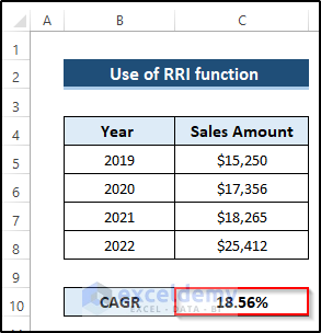
Method 4 – Using the RRI function
Steps
- To calculate the CAGR in Excel, select cell C10.
- Write down the following formula.
=RRI(3,C5,C8)
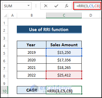
- Press Enter to apply the formula.
Breakdown of the Formula
RRI(3,C5,C8): The function returns an equivalent interest rate for the growth of an investment. 5 is the nper argument representing the number of periods, the C5 cell is the pv argument which is the Initial Value of $15250, and the C8 cell is the fv argument referring to the Final Value of $25412. The final output is 18.56%.
Method 5 – Applying the GEOMEAN Function to Compute 3-Year CAGR
Steps
- Calculate the growth factor.
- Set the growth factor 0 on cell D5, which denotes the first year of our calculation.
- Select cell D6
- Write the following formula.
=C6/C5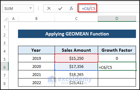
- Press Enter to apply the formula.
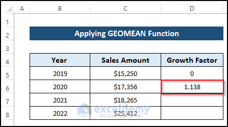
- Drag the Fill Handle icon down the column.
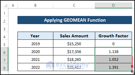
- Calculate the CAGR.
- Select cell C10.
- Write down the following formula.
=GEOMEAN(D6:D8)-1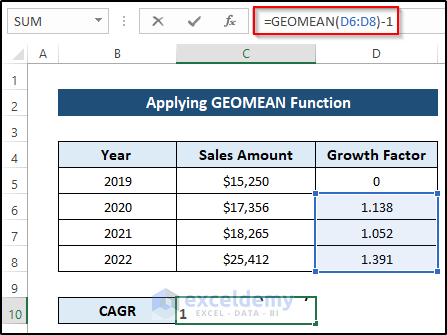
- Press Enter to apply the formula.
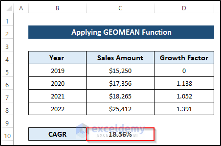
Breakdown of the Formula
GEOMEAN(D6:D8)-1: The function returns the geometric mean of an array or range of positive numbers. D6:D8 is the number 1 argument for the series of Growth Factors. Here, the output is 18.56%.
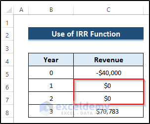
Method 6 – Utilizing IRR Function
Steps
- Insert zeros in the cells containing the intermediate Revenue values.
- Select cell C11.
- Write down the following formula.
=IRR(C5:C8)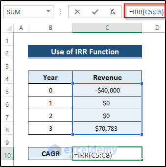
- Press Enter to apply the formula.
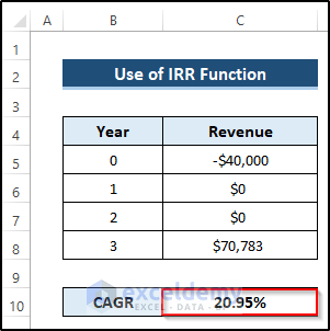
Breakdown of the Formula
IRR(C5:C8): The function returns the internal rate of return for a series of cash flows. C5:C8 is the values argument referring to the Revenues series. The output is 20.95%.
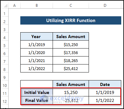
Method 7 – Applying XIRR Function to Calculate 3-Year CAGR
Steps
- Put the initial and final sales amount and dates in a different place.
- Select cell C14.
- Write down the following formula.
=XIRR(C11:C12,D11:D12)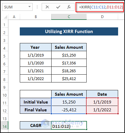
- Press Enter to apply the formula.
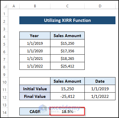
Breakdown of the Formula
XIRR(C11:C12,D11:D12): The function returns the internal rate of return for a schedule of cash flows. C11:C12 is the values argument that refers to the Initial and Final Values for the sales amount. D11:D12 represents the dates argument indicating the Initial and Final Values for the Dates.
Things to Remember
- To change the CAGR value to a percentage, press CTRL+SHIFT+”%” keys on your keyboard. Alternatively, you can open the Format Cells dialog box by pressing CTRL+1 and changing the cell formatting to a percentage.
- Excel’s compound annual growth rate formula can determine how much the investment should return annually at a constant growth rate.
- The #VALUE! error is most likely present if you encounter any Excel CAGR formula errors.
Download Practice Workbook
Download the practice workbook below.
Related Articles
<< Go Back to Compound Interest in Excel | Excel for Finance | Learn Excel
Get FREE Advanced Excel Exercises with Solutions!
