The following image is the overview of calculating compound interest.
Functions that Calculate Compound Interest for Recurring Deposits in Excel
Function 1 – FV
The FV function returns the future value of an investment based on periodic, constant payments and a constant interest rate.
Syntax of the FV function: FV(rate, nper, pmt, pv, type)
- rate: The Interest rate per period
- nper: Total number of periods
- pmt: The payment made in each period
- pv: Present value
- type: Type of payment. Payments can be of two types: the Beginning of the period (1) and the End of the period (omitted or 0).
Function 2 – EFFECT
The EFFECT function returns the effective annual interest rate.
Syntax of EFFECT Function: EFFECT(nominal_rate, npery)
- nominal_rate: Nominal Annual Interest Rate
- npery: Number of compounding will happen in a year
For example, your bank provides the Nominal Interest Rate is 6% per annum. Now you make a deposit of the amount of $100 with a bank for the next 1 year and the bank compounds your money quarterly.
What will be your effective rate or return?
Your Rate per Quarter is: 6%/4 = 1.50%. This is because your money is compounded 4 times per year. So, nominal interest is divided by 4 to get the Rate per Quarter.
Look at the image below.
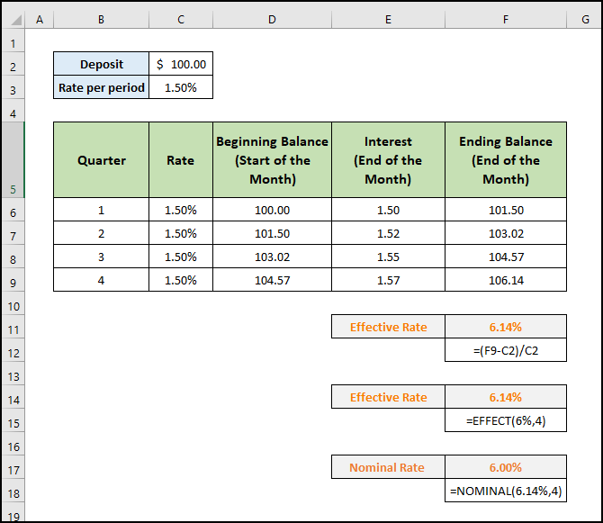
You see that:
- At the end of the first quarter, your ending balance will be $101.50. 1.50% interest is applied to the Beginning Balance of $100.
- 50 is the beginning balance at the start of the 2nd quarter. At the end of the 2nd quarter, your ending balance will be $103.02. 1.50% interest is applied on the beginning balance of $101.50
- At the end of the fourth quarter, your ending balance will be: $106.14
Your nominal interest rate is 6%. But because of 4 compoundings per year, you’re getting a 6.14% return on your investment.
We can use the EFFECT function in the cell F14 to get the above Effective Rate:
=EFFECT(6%,4)
This is shown also in the image.
Function 3 – NOMINAL
The NOMINAL function is the opposite of the EFFECT function. It returns the Nominal Interest Rate from an Effective Interest Rate.
Syntax of NOMINAL Function: NOMINAL (effect_rate, npery)
We use this function in cell F16 to get the Nominal Interest Rate from an Effective Interest Rate.
=NOMINAL(6.14%,4)
How to Calculate Compound Interest for Recurring Deposit in Excel: 2 Easy Methods
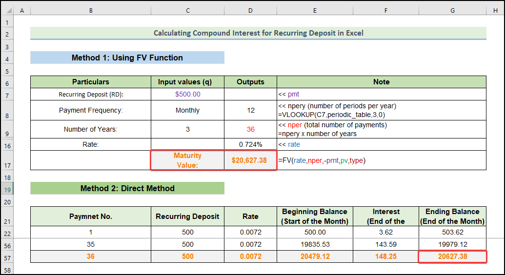
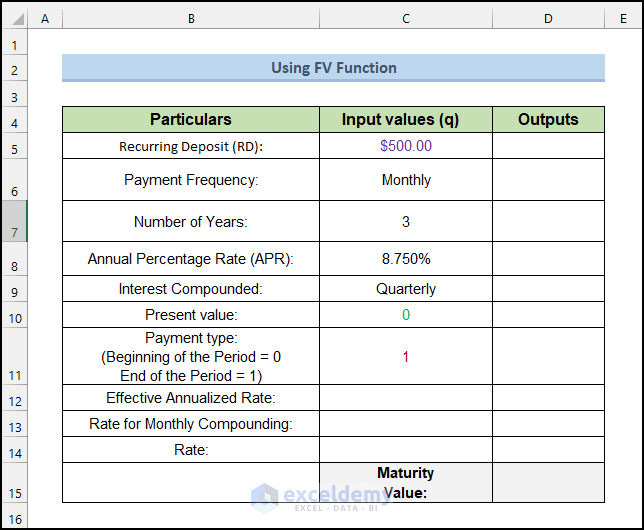
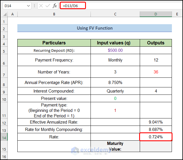
Method 1. Using the FV Function
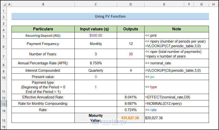
- Cell C5 is the Recurring Deposit (RD). The amount you will deposit every month (or any period). We named this cell pmt.
- Cell C6 is the Payment Frequency. It is a drop-down list. In most cases, it is monthly. But you can select any period from the drop-down.
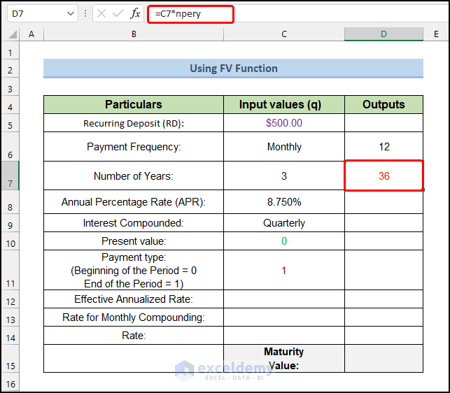
- Cell C7 indicates the Number of Years that you will keep depositing your fund. As output, we will get the total number of periods (nper) by multiplying the Number of Years by the Number of Periods per Year (npery).
- Annual Percentage Rate (APR) is represented in cell C8. This is the nominal interest rate your bank offers to you.
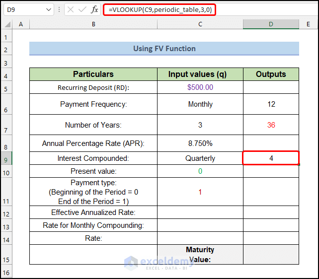
- Cell C9 illustrates the Interest Compounded. Indian Banks compound your investment quarterly. It can differ from bank to bank. This is also a drop-down list, so you can choose any compounding frequency.
Steps:
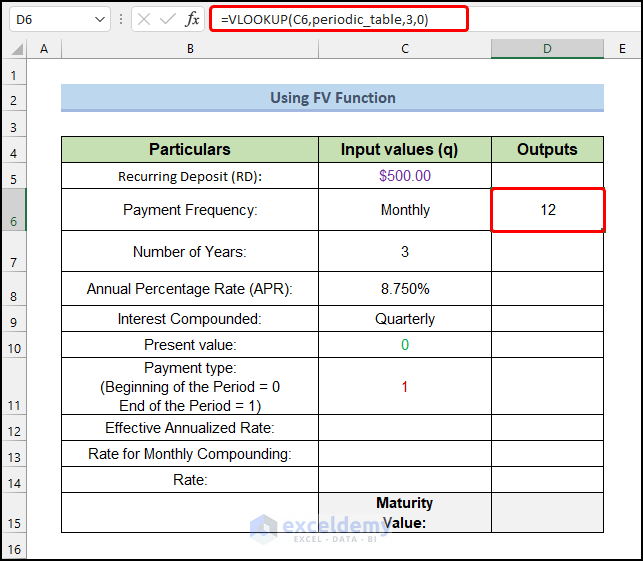
- Calculate the number of periods per year (npery) in cell D6:
=VLOOKUP(C6,periodic_table,3,0)
- Press Enter.
- The output will look like this.
- In cell D7, insert the following formula.
=C7*npery
- Press Enter.
- You will get the following output.
- For cell D9, use the following:
=VLOOKUP(C9,periodic_table,3,0)
- Press Enter.
Your Interest Compounding Frequency must be equal to or greater than the Payment Frequency. For example, if your Payment Frequency is Monthly, you cannot choose the Compounding Frequency value as Weekly, Bi-weekly, or Semi-monthly.
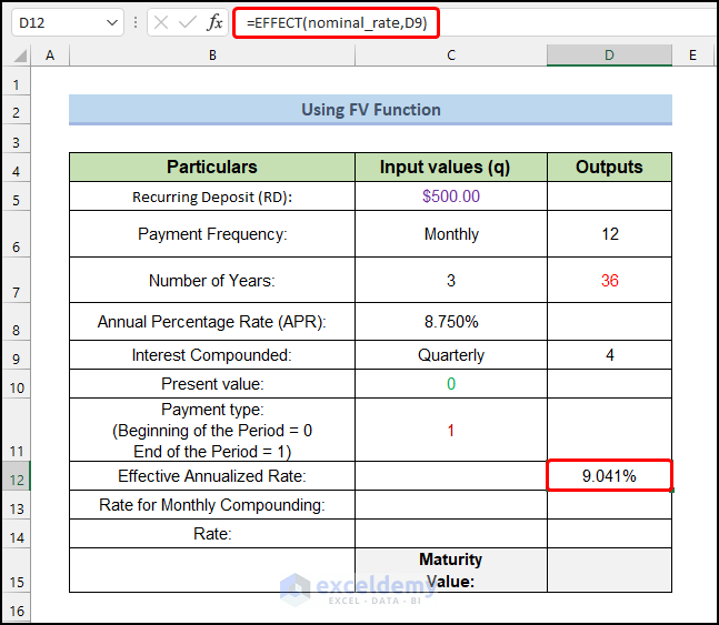
- We’ll calculate the effective rate for Quarterly compounding using the following formula:
=EFFECT(nominal_rate,D9)
- Press Enter.
- You will get the output as 9.041%.
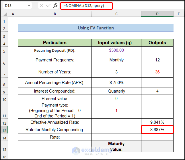
- We’ll get a nominal rate by using the following formula that will give us the same effective rate with monthly compounding:
=NOMINAL(D12,npery)
- Press Enter.
- You will get the output as 8.687%.
Note:
You can cross-check it this way: this nominal rate (8.687%) will provide the same effective rate with monthly compounding: =EFFECT(8.687%,12) =9. 041%.
- Get the rate for a period (monthly) using the following formula.
=D13/D6
- Press Enter.
- You will get the output as 0.724%.
- Use the FV function in cell D16 to the maturity value. The formula is as follows:
=FV(rate,nper,-pmt,pv,type)
- Press Enter.
- You will get the output as $20,627.38.
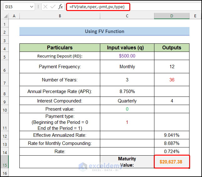
- The following image shows the whole process that we have used to calculate the recurring deposit.
Read More: Formula for Monthly Compound Interest in Excel
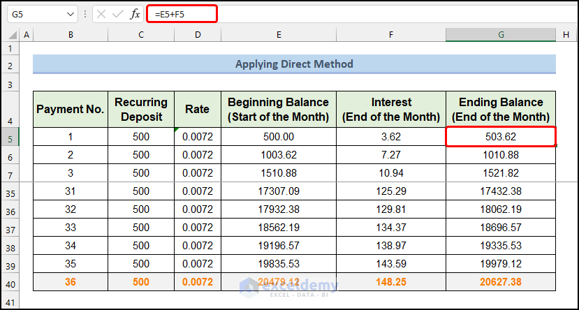
Method 2 – Applying the Direct Method
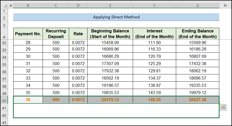
This is a step-by-step calculation to get the Maturity Value of your Recurring Deposit (RD) for 36 periods (3 years).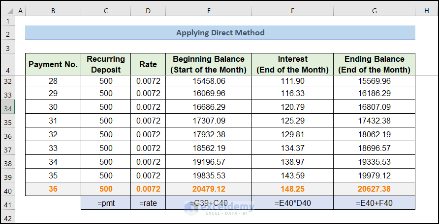
Steps:
- Type the serial number of the payment in column Payment No.
- We have used the same pmt value in the Recurring Deposit column, and the same rate per period in the Rate column.
- Enter the recurring deposit value in cell E5.
- Enter the following in cell E6 to calculate the beginning balance:
=G5+C6
- Press Enter.
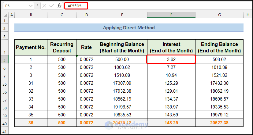
- Copy the following in cell F5 to calculate the interest:
=E5*D5
- Press Enter.

- Insert the following in cell G5 to calculate the ending balance:
=E5+F5
- Press Enter.
- The Maturity Value of our Recurring Deposit for 36 periods (3 years) will be 20,627.38, which is the same value as the FV function’s method.
- To add more periods to this table, copy the last row down as needed.
Read More: Methods to Apply Continuous Compound Interest Formula in Excel
Download the Practice Workbook
Download the Excel workbook that can also be used as a template.
Related Article
<< Go Back to Compound Interest in Excel | Excel for Finance | Learn Excel
Get FREE Advanced Excel Exercises with Solutions!

Thank you for this useful article. The maturity does tally with the Indian banks (e.g. Axis Bank) as calculated in the Bank’s website.
You can use this formula to calculate PPF interest.
can I use this formula to calculate PPF interest?
Hi SANSHI,
You can use the direct method to calculate the PPF interest easily.
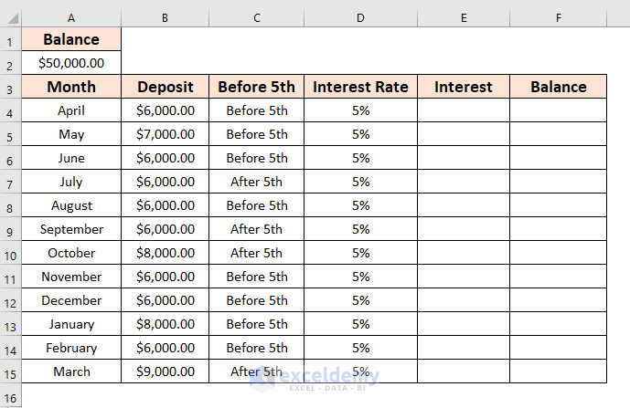
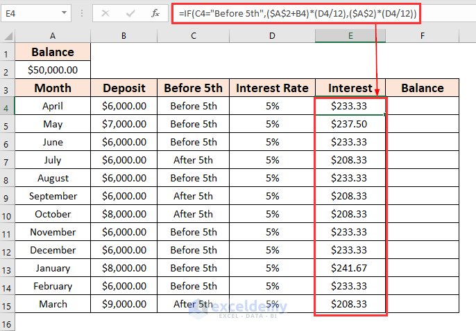
For calculating the PPF interest, we will be using the following dataset. Here, we have the total Balance, Deposits from April to March, and an Interest Rate of 5%.
• For the monthly interest rates use the following formula
=IF(C4=”Before 5th”,($A$2+B4)*(D4/12),($A$2)*(D4/12))
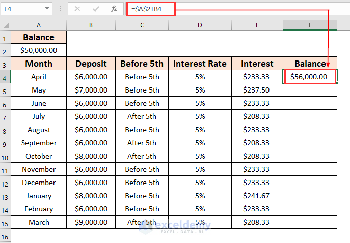
• For the first month of getting the balances, apply the following formula in cell F4.
=$A$2+B4
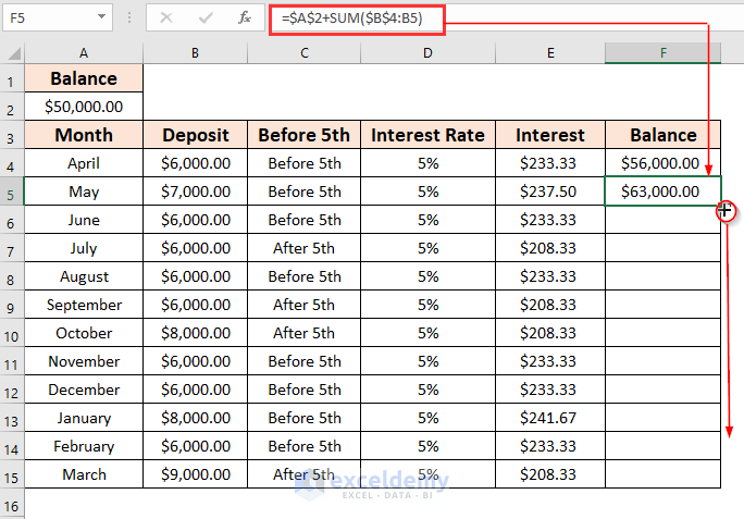
• To get the rest of the balances type the following formula
=$A$2+SUM($B$4:B5)
• Drag down the Fill Handle tool.
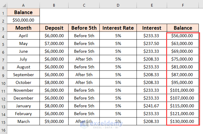
The final output will look like the following figure.