How to calculate compound annual growth rate (CAGR) in Excel (7 Methods)

Method 1 – Calculating CAGR with a Generic Formula

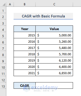
The following dataset contains some compounded amounts over successive years. The initial value is $5000, which has been compounded to $6850 after a period of 6 years. Using these values, we’ll calculate the CAGR with a generic formula.

Steps:

• Enter the following formula in Cell C13:

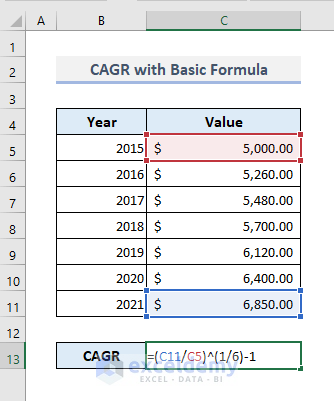
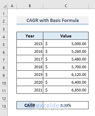
• Press Enter and change the number format to a percentile. We’ll get a return value of 5.39%.

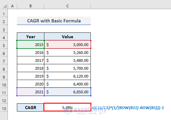
The number of total periods is the subtraction between the final and the beginning years for our dataset. So, for a large number of periods, it could be quite exhausting to count them manually. In this case, using the subtraction formula between the row numbers for the beginning and final years would be better. We can use the ROW function here to input the row numbers in the subtraction formula to count the number of compounding periods.

• Use the ROW function to define the number of periods, the modified formula would look like the following:

The resultant value is the same as found earlier.

Method 2 – Using the POWER Function to Determine CAGR in Excel

The POWER function returns the result of a number raised to a power. The syntax of this function is as follows:

=POWER(number, power)

Where,

number = A valid numeric value.

power = The power (index) to be applied to the numeric value (base).

Using this simple POWER function, we can easily define the ratio of the future value and initial value along with the number of total periods (months, years).

Steps:

To calculate CAGR with the use of the POWER function,

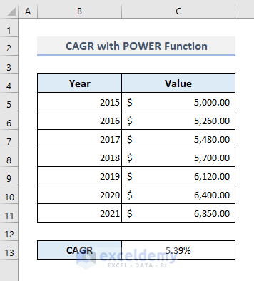
• Enter the following formula in Cell C13:

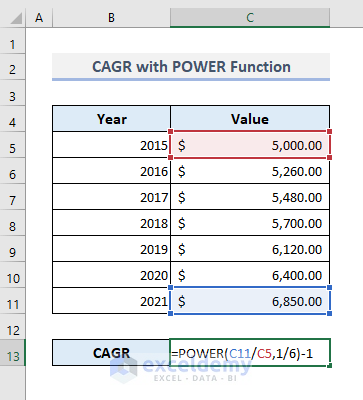
• Press Enter, and we’ll get a similar result value to the one found in the previous method.

Read More: How to Calculate CAGR with Negative Number in Excel

Method 3 – Using the Excel RATE Function

The RATE function returns the interest rate per loan or investment period. The syntax of this function is:

=RATE(nper, pmt, pv, [fv], [type], [guess])

Here,

nper = Number of total periods (in years or months).

pmt = Additional payment in each period.

pv = Present Value, known as Initial investment value.

[fv] = Option argument, denotes the Future Value of an investment.

[type] = Optional value. ‘0’ refers to the due payments at the beginning and ‘1’ refers to the due payments at the end.

[guess] = Optional argument, means estimated guess of the rate. If omitted, the default value will be 10% for this argument.

Steps:

To calculate CAGR with the RATE function, we have to use only three arguments: nper, pv, and [fv]. Here, the pv (Present Value) must be negative; otherwise, the function will return a #NUM error.

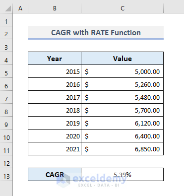
• Enter the following formula in Cell C13:

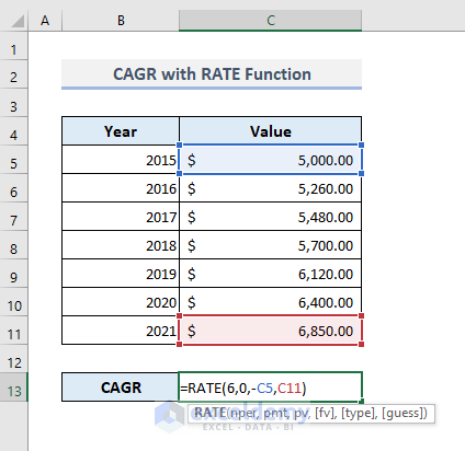
• Press Enter to get the return rate as 5.39%.

Method 4 – Inserting IRR Formula to Find Out CAGR in Excel

The syntax of the IRR function is:

=IRR(values, [guess])

Here,

values = Range of cells or an array containing numeric values.

[guess] = Optional argument. An estimation of the interest rate, if omitted, the default will be 10%.

We can also calculate the CAGR using this IRR function. However, you must maintain some criteria while inputting the arguments.

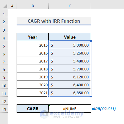
In the following dataset, the compounded growths of the initial investment value have been displayed over many periods by year. If we input the investment value with all chronic growths in the IRR function, the function will return a #NUM! error. It’s because the initial value in the range of cells must be negative.

• Make the first numeric value or the initial investment in Cell C5 negative.

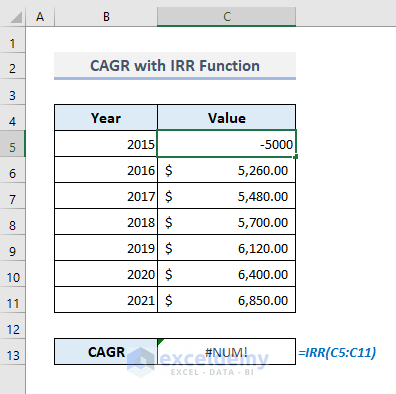
• Press Enter, and you’ll get a CAGR of 108.10%! But we need to get 5.39%.

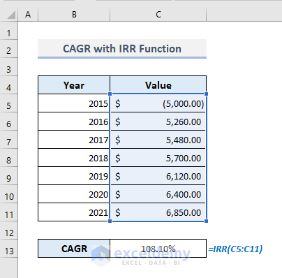
The problem with the formula is that, along with the initial value, we have entered all compounded amounts in the selected range of cells (C5:C11). Still, this function has counted these positive values as additional payments. So, we cannot use this sort of range of cells where all compounded values are present. Rather, we have to use only the range of cells containing an initial value and a future value.

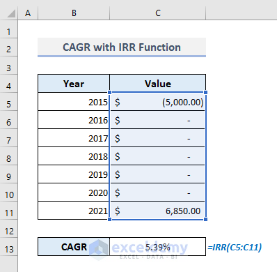
If we remove all intermediate amounts from the selected range of cells, the function will return an accurate compound annual growth rate of 5.39%. The first value in the range of cells must be a negative number.

Read More: Excel Formula to Calculate Average Annual Compound Growth Rate

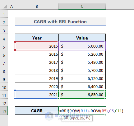
Method 5 – Using the RRI Function to Calculate CAGR

The syntax of this RRI function is:

=RRI(nper, pv, fv)

Where,

nper = Number of total periods (in years or months).

pv = Present value or the initial investment.

fv = Future value or the final compounded amount after a certain period.

• The required formula with the RRI function based on our dataset to find out CAGR will be:

We’ve used the ROW functions in this formula to assign the total number of periods.

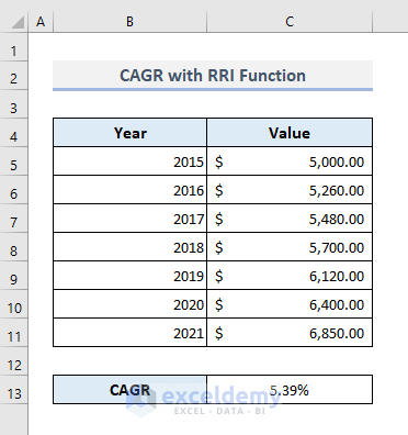
• Press Enter, and the formula will return the CAGR of 5.39%, as found in all other previous methods.

Read More: How to Calculate Future Value When CAGR Is Known in Excel

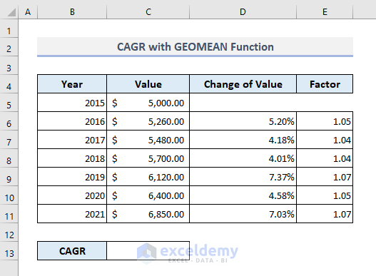
Method 6 – Using the Excel GEOMEAN Function

The generic formula of this function is as follows:

=GEOMEAN(number1, [number2],…)

To determine the CAGR with the GEOMEAN function, we must add two more columns, as shown in the following image. The Change of Value column shows the percentage change of each preceding value from the Value column. The Factor column represents all the growth factors we found by adding ‘1’ to each percentage change.

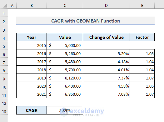
To calculate the CAGR with the GEOMEAN function,

• Enter the following formula in Cell C13:

• Press Enter, and we’ll get the growth rate of 5.39%.

Method 7 – Entering the XIRR Function to Determine CAGR with Non-Periodic Cash Flows

The XIRR function returns the internal rate of return for a schedule of cash flows. The syntax of this XIRR function is:

=XIRR(values, dates, [guess])

Here,

values = Range of cells containing all cash flows.

dates = Corresponding dates for the cash flows.

[guess] = An estimated rate of return; if omitted, the default value is 10%.

In the modified dataset below, several cash flows are present with their corresponding dates. The first value in the Value column is negative because this amount of money was initially withdrawn. The rest of the values are positive as they’re all deposited amounts. The cash flows were recorded between 26 January 2021 and 26 January 22.

To find out the CAGR associated with the mentioned data,

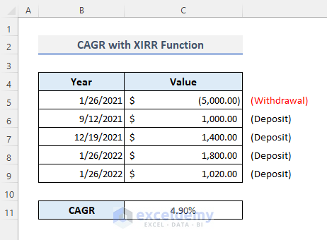
• Enter the following formula with the XIRR function in Cell C11:

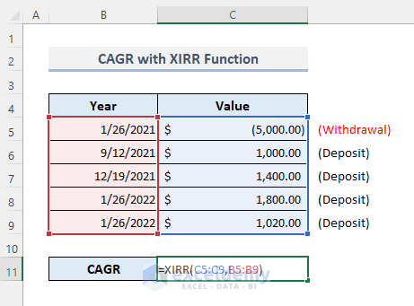
• Press Enter to get a return value of 4.90% for all non-periodic cash flows.

Read More: How to Calculate End Value from CAGR in Excel

Online Calculator with CAGR Formula

In the downloadable Excel workbook attached to this article, you’ll find the templates with all the formulas and methods described so far. You can use those templates as calculators where you’ll find all possible criteria to input.

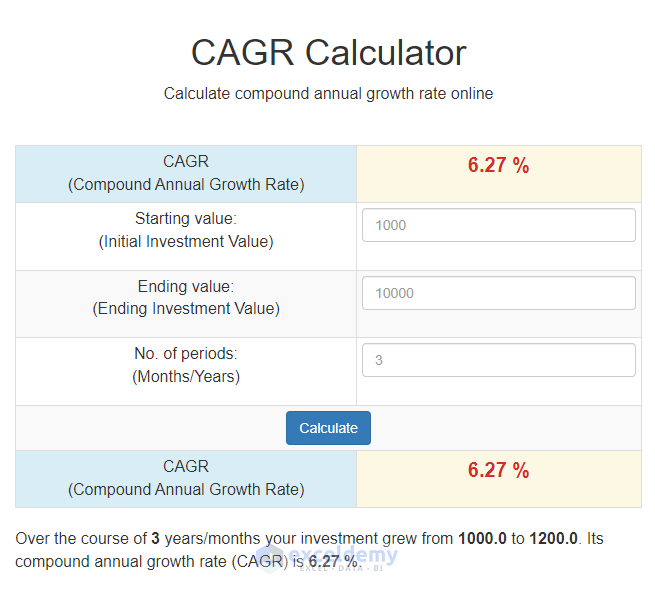
If you prefer to avoid Excel spreadsheets, you can also look for a CAGR calculator online. I recommend the CAGRCalculator website. Their online calculator contains all possible input criteria. You can also find the future value, internal rate of return, and initial investment amount with other calculators associated with the compound interest formulas.

The following screenshot is an overview of the interface of their CAGR calculator. You have to input the starting value, ending value, and the no. of periods only in the corresponding sections.

The calculator also returns the growth table for the compounded values over all periods.

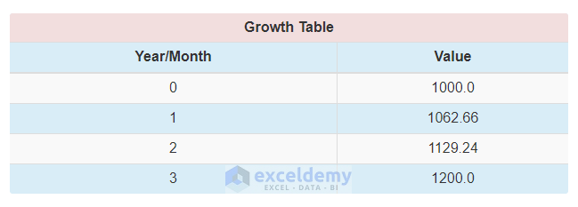
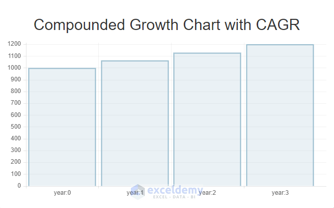
You’ll find a graphical chart showing year-by-year compounded amounts.

Things to Keep in Mind

• While using the RATE function to determine CAGR, the argument pv (Present Value) will be negative.
• The argument pv will be positive in the RRI function.
• The first or initial value for the IRR function has to be negative.
• In the XIRR function, the cash flows must contain at least one negative value; otherwise, it will return a #NUM! error.
• For non-periodic cash flows, the percentage of CAGR for a similar future value won’t be identical to the CAGR calculated for the periodic cash flows.

Download the Practice Workbook

You can download our Excel workbook to practice.

Related Articles

• How to Calculate 3-Year CAGR with Formula in Excel
• How to Calculate 5 Year CAGR Using Excel Formula
• How to Create CAGR Graph in Excel

<< Go Back to Compound Interest in Excel | Excel for Finance | Learn Excel