How to Calculate 5 Year CAGR Using Excel Formula

Excel is a popular and useful tool for modeling growth and analyzing data. One such case is the calculation of CAGR. In this regard, Excel becomes a handy tool to perform such calculations effortlessly. Keeping this in mind, this article demonstrates 7 useful ways how to calculate 5 year CAGR using formula in Excel.

What Is CAGR?

First of all, let’s dwell a little upon what “CAGR” is.
CAGR stands for Compound Annual Growth Rate which is a measure of growth on the assumption that it compounds at a constant rate over a specified period of time. Typically, financial professionals use CAGR to evaluate and contrast numerous possibilities and come to a more informed decision.

Formula to Calculate CAGR in Excel

Now, the formula to calculate the CAGR is as follows:

where,

• Final Value is the closing value of the growth model.
• Initial Value refers to the beginning value of the model.
• Year represents the time interval in years, months, quarters, etc.

Calculate 5 Year CAGR Using Formula in Excel: 7 Ways

Suppose consider the Yearly Growth Rate of the ExcelDemy Subscribers dataset shown in the B4:C10 cells, which shows the Year and Number of Subscribers respectively. Here, we want to calculate the Compound Annual Growth Rate of this data model, therefore, without further delay let’s explore all the nitty-gritty of each method with appropriate illustrations.

Here, we have used the Microsoft Excel 365 version, you may use any other version according to your convenience.

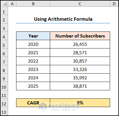
Method 1: Using Arithmetic Formula

First and foremost, let’s kick things off by applying the arithmetic formula of CAGR in Excel.

📌 Steps:

• At the very beginning, go to the C12 cell >> and enter the formula given below.

Here, the C5 and C10 cells refer to the Initial and Final Values while the 5 represents the Year.

📃 Note: Please make sure to press the CTRL + SHIFT + % keys on your keyboard to change the CAGR value to a percentage.

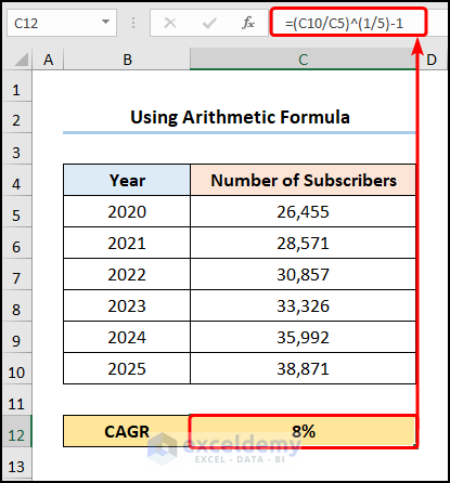
That’s it. You’ve calculated the 5 year CAGR formula in Excel. It’s that simple!

Method 2: Utilizing the RATE Function

If you’re one of those people who enjoy using Excel functions, then the following methods have you covered. On this occasion, we’ll use the RATE function to calculate the growth rate of the subscribers and the ROW function to return the Initial and Final Values. So, let’s see it in action.

📌 Steps:

• In the first place, move to the C12 cell >> type in the equation given below.

In the above equation, the C5 and C10 cells indicate the Initial and Final Values while the 5 represents the Year.

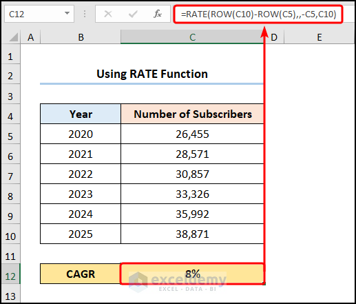
Finally, the results should look like the image shown below.

Read More: CAGR Formula in Excel

Method 3: Applying POWER Function

Alternatively, we can apply the POWER function to compute the 5-year CAGR formula of the growth model. For instance, the POWER function returns the result of the ratio of the Final to Initial Value raised to the reciprocal of the Year value.

📌 Steps:

• Initially, navigate to the C12 cell >> insert the following expression.

In this expression, the C5 and C10 cells point to the Initial and Final Values respectively whereas, 5 refers to the Year value.

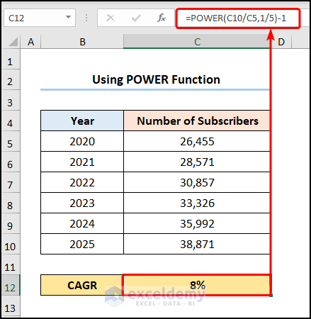
Finally, the output should look like the screenshot given below.

Read More: How to Calculate End Value from CAGR in Excel

Method 4: Using RRI Function

Normally, the RRI function estimates the corresponding interest rate for the growth of an investment. However, it can also be used to calculate the compound annual growth rate. It’s simple and easy; just follow along.

📌 Steps:

First, insert the following formula into the C12 cell.

Specifically, the C5 and C10 cells represent the Initial and Final Values, in contrast, 5 is the number of Years.

📃 Note: You can open the Format Cells dialog box by pressing CTRL + 1 and changing the cell formatting to percentage.

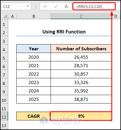
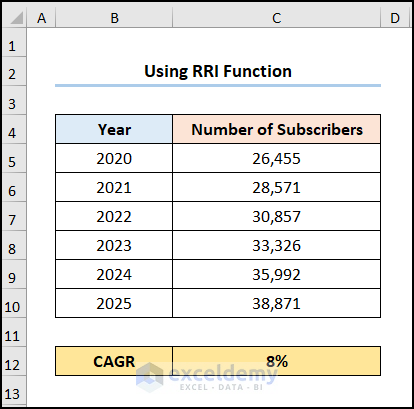
Subsequently, your result should look like the image shown below.

Read More: How to Calculate Future Value When CAGR Is Known in Excel

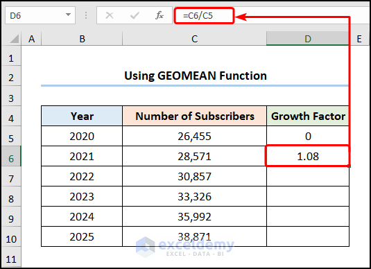
Method 5: Applying the GEOMEAN Function

Conversely, we can use the GEOMEAN function to enter a series of Growth Factors and obtain the geometric mean of this array which is the CAGR value. Now, allow me to demonstrate the process in the steps below.

📌 Steps:

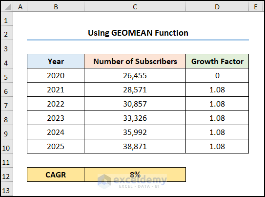
• To begin with, go to the D6 cell >> enter the formula given below.

In this case, the C5 and C6 cells represent the Number of Subscribers for the Years 2020 and 2021.

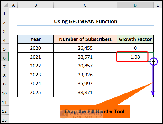
• Then, use the Fill Handle Tool to copy the formula into the cells below.

• Next, insert the GEOMEAN function into the C12 cell.

For instance, the D6:D10 series points to the Growth Factor values for the Years 2021 to 2025.

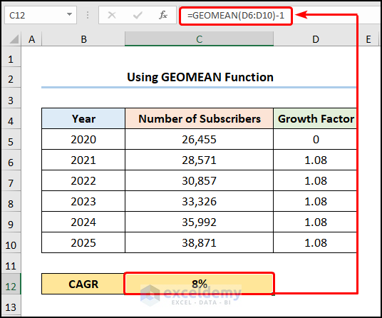
Ultimately, the output should appear in the picture shown below.

Read More: Excel Formula to Calculate Average Annual Compound Growth Rate

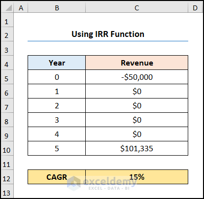
Method 6: Employing IRR Function

Although the IRR function calculates the internal rate of return for a series of cashflows, it can be re-purposed to get the CAGR value. However, we have to manipulate the dataset to get the desired results. Hence, let’s see the process in detail.
Now, assuming the Yearly Growth Rate of Revenue dataset shown in the B4:C11 cells, which shows the Year and Revenue respectively.

📌 Steps:

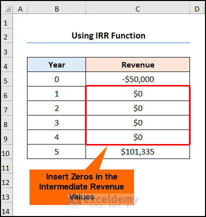
• To start, insert zeros in the cells containing the intermediate Revenue values.

• Later, copy and paste the expression into the Formula Bar.

In this situation, the C5:C10 array indicates the Revenue values for the Years 0 through 10.

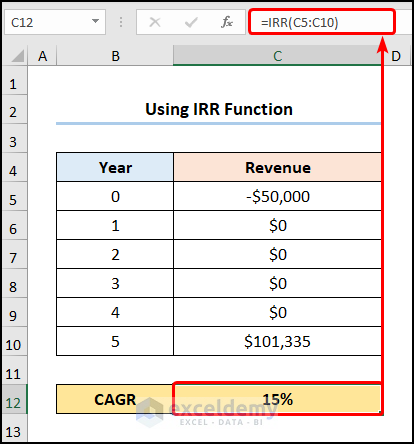
Consequently, the CAGR value should be equal to 15%.

Method 7: Utilizing the XIRR Function

Last but not least, we’ll employ the XIRR function which returns the non-periodic cash flows, so we’ll modify our existing dataset to show the Dates instead of the Year, such that we can compute the CAGR value.

📌 Steps:

• First, proceed to the C16 cell >> type in the equation given below.

For example, the C13:C14 and D13:D14 range of cells refer to the Initial and Final Values corresponding to the Number of Subscribers and the Date.

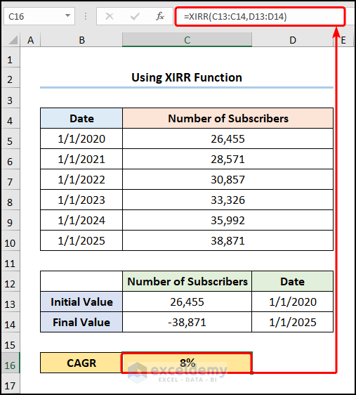
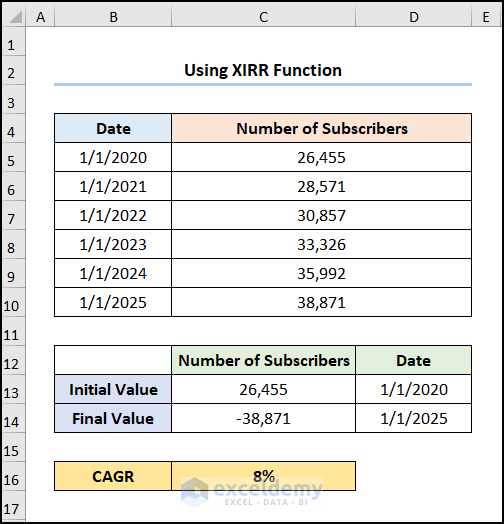
Eventually, the results should look like the picture given below.

Read More: How to Calculate CAGR with Negative Number in Excel

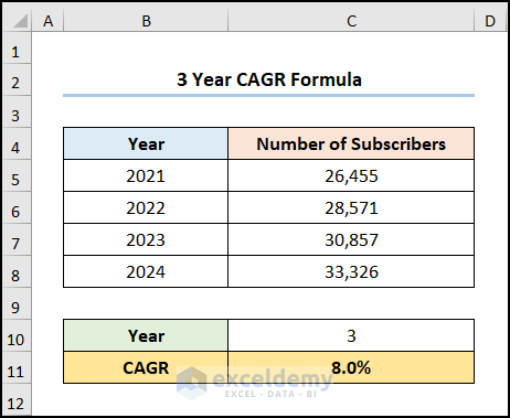
How to Calculate 3-Year CAGR Using Formula in Excel?

So far, we’ve discussed the 5-year CAGR formula in Excel. If you want to obtain the CAGR for a different number of years, for instance, 3 years, the following section answers this exact question. In this case, we’ll apply the COUNT function to count the number of years in the dataset and obtain the CAGR value with the RRI function. So, follow along.

📌 Steps:

In the first place, enter the formula into the C10 cell.

Here, the B5:B8 cells represent the number of Years.

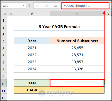
• In turn, type in the RRI function in the C11 cell as shown below.

On this occasion, the C5 and C8 cells represent the Initial and Final Values and the C10 cell is the Year value.

📃 Note: You can press CTRL + SHIFT + %  shortcut to change the cell formatting to percentage.

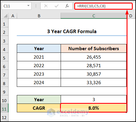
Finally, your output should look like the screenshot given below.

Practice Section

We have provided a Practice section on the right side of each sheet so you can practice yourself. Please make sure to do it by yourself.

Download Practice Workbook

Conclusion

To sum up, this article shows 7 effective methods on how to calculate 5-year CAGR using formulas in Excel. So, read the full article carefully and download the free workbook to practice. Now, we hope you find this article helpful and if you have any further queries or recommendations, please feel free to comment here.

Related Articles

• How to Calculate 3-Year CAGR with Formula in Excel
• How to Create CAGR Graph in Excel

<< Go Back to Compound Interest in Excel | Excel for Finance | Learn Excel