Compound Interest with Monthly Compounding Periods
Compound interest is the total interest that includes the original interest and the interest of the updated principal which is evaluated by adding the original principal to the due interest. It is the interest that you get both on your initial principal and on the interest you earn with the passage of each compounding period. When the interest is compounded after each of the 12 months, it is called monthly compound interest.
Basic Mathematical Formula:
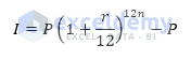
I = Compound interest.
P = Original principal.
r = Interest rate in percentage per year.
n = Time in years.
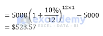
Mathematical Example:
A borrower took a $5000 loan at a 10% annual interest rate for 5 years.
The monthly compound interest will be
Formula 1 – Calculate Monthly Compound Interest Manually in Excel Using the Basic Formula
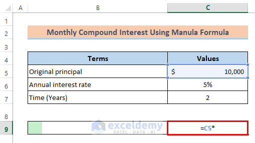
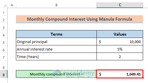
A client borrowed $10000 at a rate of 5% for 2 years from a bank. To find the monthly compound interest: 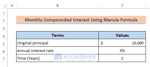
Steps:
- C5 contains the original principal (Present value). Multiply this value by the interest rate. Enter:
=C5*
- Divide the annual interest rate by 12.
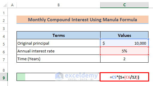
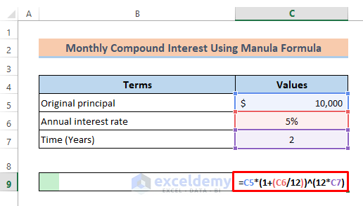
- Provide a cell reference with the number of years to multiply the value by 12. The formula becomes
=C5*(1+(C6/12))^(12*C7).
- Subtract C5 which contains the original principal. The formula becomes-
=C5*(1+(C6/12))^(12*C7)-C5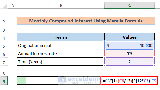
- Press Enter.
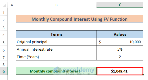
The monthly compound interest is displayed.
Read More: Methods to Apply Continuous Compound Interest Formula in Excel
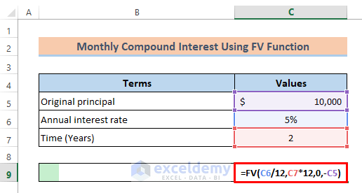
Formula 2 – Use the Excel FV Function to Calculate the Monthly Compound Interest
Syntax of FV Function:
=FV(rate,nper,pmt,[pv],[type])Arguments:
rate(required argument) – The interest rate per period.
nper (required argument) – The total payment periods.
pmt (optional argument) – It specifies the payment per period. If this argument isn’t used, the PV argument must be provided.
[pv](optional argument) – It specifies the present value (PV) of the investment. If it is omitted, it defaults to zero and the Pmt argument must be provided.
[type] (optional argument) – It identifies whether the wages are created at the start or at the end of the year. It will be 0 at the end, and 1 at the start.
Steps:
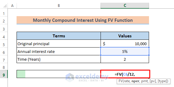
- Specify the rate in the FV function. Divide the annual rate by 12: enter
=FV(C6/12,in C9.
- Specify the total periods. Multiply the time in years(C7) by 12.
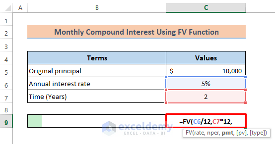
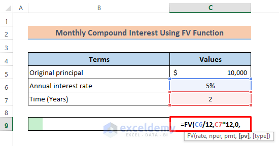
- As no additional amount is added to the original principal value in between the investment period, ‘0’ is used for ‘pmt.’ The formula becomes
=FV(C6/12,C7*12,0,.
- As $10000 as the original principal is invested and the value for ‘pmt’ is omitted, the cell reference C5 is used with a negative (-) sign. Enter:
=FV(C6/12,C7*12,0,-C5).
- Subtract the original principal from the future value to get the interest. Enter the formula:
=FV(C6/12,C7*12,0,-C5)-C5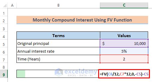
- Press Enter.
Read More: How to Calculate Compound Interest for Recurring Deposit in Excel
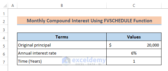
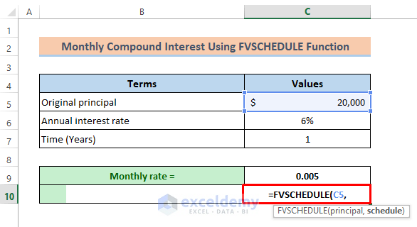
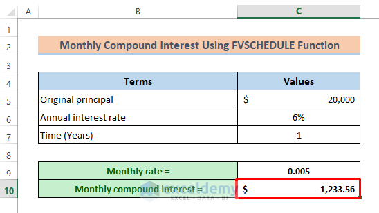
Formula 3 – Apply the Excel FVSCHEDULE Function to Calculate the Monthly Compound Interest
Syntax of FVSCHEDULE Function:
=FVSCHEDULE(principal, schedule)Arguments:
Principal (required argument) – The present value of the investment.
Schedule (required argument) – The array of values that provides the schedule of interest rates to be applied to the principal.
The dataset was modified.
- Enter the present value in the FVSCHEDULE function:
=FVSCHEDULE(C5,in C10.
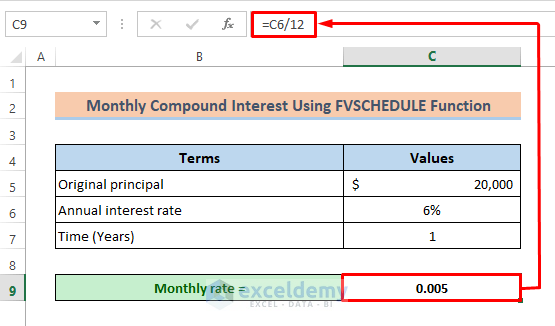
- Set the schedule of interest rates as an array. Divide the annual rate by 12 in C9.
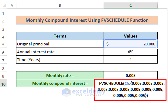
- Enter this value 12 times as an array in the formula. Enter:
=FVSCHEDULE(C5,{0.005,0.005,0.005,0.005,0.005,0.005,0.005,0.005,0.005,0.005,0.005,0.005}).
- Subtract the original principal. The final formula is:
=FVSCHEDULE(C5,{0.005,0.005,0.005,0.005,0.005,0.005,0.005,0.005,0.005,0.005,0.005,0.005})-C5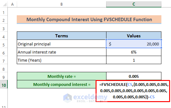
- Press Enter.
Download Practice Workbook
Download the free Excel template here and practice.
Related Article
<< Go Back to Compound Interest in Excel | Excel for Finance | Learn Excel
Get FREE Advanced Excel Exercises with Solutions!

How can you calculate monthly interest where you have the principal and every month you save ?
Dear Emely Phiri,
Thanks for reaching out to us. Let’s clear your confusion.
Think of it this way, you already know how one can calculate annual interest when one has the principle and the every month’s saving’s amount. If it is simple interest, you use the I=P*r*n formula and for compound interest, you use I=P*(1+r)^n-P.
Now, if I say, your principle is $1200, interest rate is 10% then the annual interest using the simple formula would be $1200*0.1*1=$120 right? Which means, the interest you are actually getting is $120/12=$10 every month. And if you save like $50 every month, the total amount in your account at the end of the first month and at the beginning of the second month will be $1200+$10+$50=$1260, where $1200 is your principle, $10 is the first month’s interest and $50 is the amount you further deposited into your account.
Now, as you have deposited $50 more, would the interest at the end of the second month and at the beginning of the third month be the same? Of course not.
At the beginning of the second month, the net amount in your account is $1260 right? Then, as the interest rate is 10%, so in that sense the annual interest using this new amount should be $1260*0.1*1=$126. So basically, the monthly interest this time becomes $126/12=$10.5. That means, at the end of the second month and at the beginning of the third month, the net amount in your account now is $1260+$10.5+$50=$1320.5, where $1260 is the net amount at the beginning of the second month, $10.5 is the monthly interest and $50 is the amount you save every month. And the same procedure goes on for the rest of the months as you are depositing money every month into your account.
For monthly compound interest, the procedure is mentioned in this article.
Hope, this clears your confusion. Have a great day.