This article will focus on using an Excel formula consisting of the FVSCHEDULE function. This function is used to calculate the future value of a payment, loan, or asset for changing interest rates. In real life, the varying interest rate is a pretty common occurrence with inflation and other causes. So this function is a handy one when it comes to calculating future values of a current asset in these scenarios.
Overview of FVSCHEDULE Formula
⏺ Function Objective
While the FV function is widely used to calculate future values in a payment or scheme, it only considers a fixed rate for both increases and decreases in values. However, what happens if the interest rate is variable or not fixed? In cases like these, in order to calculate the future value, we have to use the FVSCHEDULE Function.
⏺ Syntax
=FVSCHEDULE(principal,schedule)
⏺ Arguments Explanations
| Argument | Required/Optional | Explanation |
|---|---|---|
| principal | Required | This is the present value. |
| schedule | Required | It is a series or array of differing interest rates to apply. |
⏺ Returns
It returns the future values of the irregular payments.
From the previous section, we can see that, we only need two arguments for formulas consisting of the FVSCHEDULE function in Excel. We just need the value of the present value of the payment and the interest rates as an array. Then we can use the function just like any other function in Excel.
Let’s take a look at the following example.
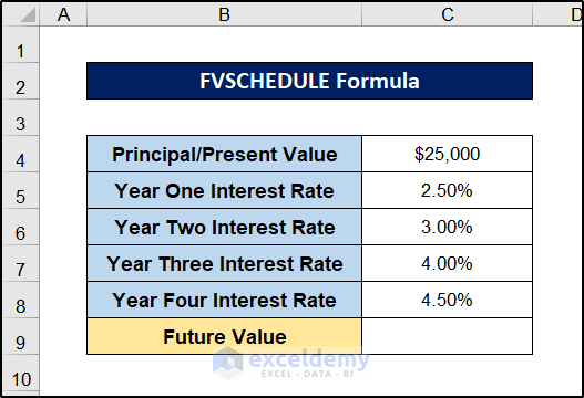
In this dataset, we have four changing interest rates for each year. For cases like these, we can use a formula consisting of the FVSCHEDULE function to determine the future value of the principal easily in Excel.
Follow these steps to see how we can do so for this dataset.
Steps:
- First of all, select cell C9.
- Then write down the following formula in the cell.
=FVSCHEDULE(C4,C5:C8)
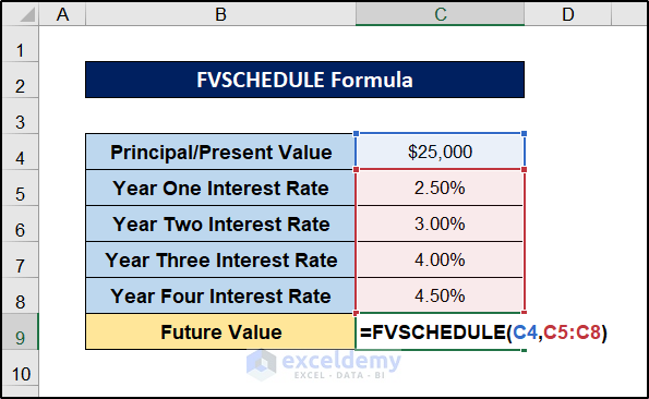
- After that, press Enter on your keyboard.
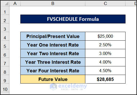
That’s all you need to do to find the future value of a payment. Here, the value in cell C9 is the future value of the principal of $25000 with these interest rates.
Now we will be showing two more practical cases of the usage of the formula consisting of the FVSCHEDULE function in Excel. We will be using different datasets for each one and a slightly different approach to using the same function.
1. Using FVSCHEDULE Formula with Excel Cell References
In the first example, we are going to use the FVSCHEDULE function with cell references just like any formula used in Excel. For this example, we will be using the following dataset.
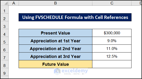
The appreciation in real estate indicates an increase in values. This works the same as an interest rate. This is a case where the increase isn’t fixed each year and a perfect example of the practicality of using functions like FVSCHEDULE.
Follow these steps to determine the future value of the property after three years with these appreciations.
Steps:
- First, select cell C8.
- Second, write down the following formula in the cell.
=FVSCHEDULE(C4,C5:C7)
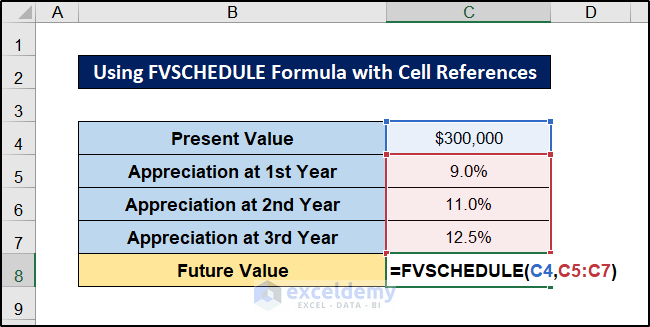
- Finally, press Enter on your keyboard.
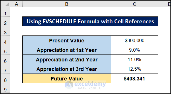
This is how we can use the formula consisting of the FVSCHEDULE function in Excel with cell references.
2. Applying Excel FVSCHEDULE Formula with Array
Now we will use the same formula, but this time by manually entering the input values. For that, we need to use an array consisting of the interest/appreciation values as the schedule argument for the formula.
For example, let’s take a look at the following dataset.
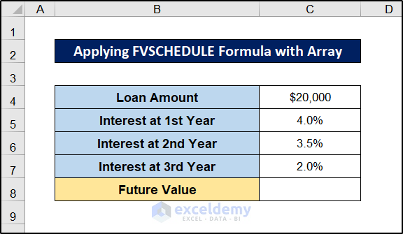
The value for the second argument should be {0.04,0.035,0.02} for this dataset. Follow these steps for a detailed guide to the procedure.
Steps:
- First, select cell C8.
- Then write down the following formula in it.
=FVSCHEDULE(C4,{0.04,0.035,0.02})
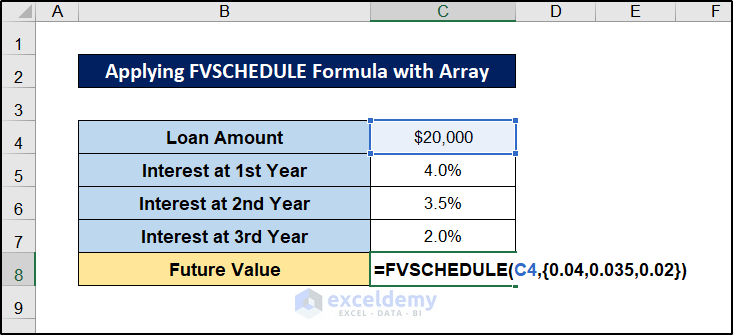
- Finally, press Enter on your keyboard.
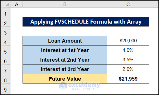
This is how we can find the future value from varying interest rates using the formula of the FVSCHEDULE function in Excel using the array.
Things to Remember
👉 If you do not use the cell reference, make sure to put the values of the second argument in an array. Always put curly braces to start and end the array.
👉 All the values in the arguments of the function should be of numeric values. Otherwise, it will return an error.
👉 If there are any blank cells in the array, the function will work fine. As there was no value involved, it will work as though there was a zero on the spot.
Download Practice Workbook
You can download the workbook used for a demonstration from the link below.
Conclusion
That concludes the usage of the FVSCHEDULE function formula in Excel. Hopefully, you have grasped the idea of using the function and can use the function for your own purposes. I hope you found this guide helpful and informative. If you have any questions or suggestions, let us know in the comments below.
<< Go Back to Excel Functions | Learn Excel
Get FREE Advanced Excel Exercises with Solutions!
