You may have created Chart in Excel on the basis of some gathered data. But sometimes you may need to create a chart with a dynamic date range to evaluate data over a certain period of time. In this article, I will show you how to create a chart with a dynamic date range in an Excel Spreadsheet.
How to Create Chart with Dynamic Date Range in Excel: 2 Easy Ways
In this section, you’ll find 2 easy ways for making a chart with a dynamic date range in an Excel workbook by using Excel built-in features and formulas. Let’s check them now!
1. Interactive Date Range Chart Technique for Dynamic Range
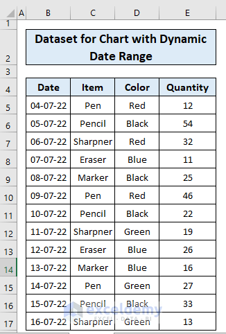
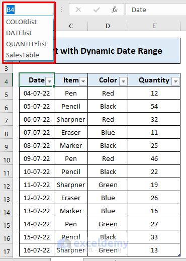
Let’s say, we have got a dataset for various items of a shop, their colors, and the quantity of sales over a certain period of time.
Creating Dynamic Range
Dynamic Ranges can be created in two ways.
i) Naming Table
ii) OFFSET Function
Naming Table
To create a chart with a dynamic date range by using the Naming Table method, just follow the steps below:
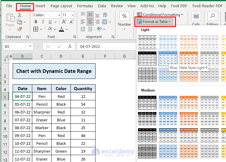
- At first, select any of the cells, go to the Home tab and click Format as Table > choose a format.
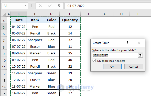
- Then assign the data range and click OK.
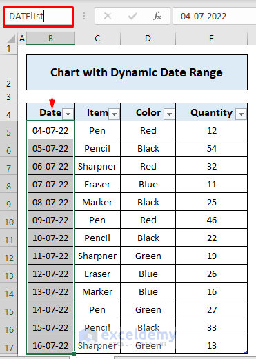
- After that, a table will be created. Select any cell and go to the Table Design tab> assign a new Table Name. We have given the name Sales Table.

- Now, take the cursor to the top edge of the cell describing Date and the whole column containing data will be selected. Give a new one-word name(i.e. DATElist) to this in the name box.
- However, repeat this step to give names to the other columns. After assigning names, you can see them by clicking the cell name just like in the screenshot below.
OFFSET Function
You can also create a dynamic range by the OFFSET Function. For this, just follow the steps below:
- Firstly, go to the Formulas tab on the ribbon> click Define Name.

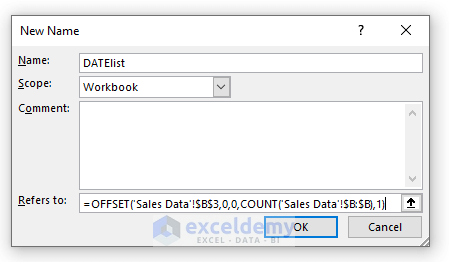
- Then, a dialogue box will show up. Assign a name for the first range(i.e. DATElist) and enter the following Formula to the Refres to box:
=OFFSET(Sales Data!$B$3,0,0,COUNT(Sales Data!$B:$B),1)Here,
- Sales Data!$B$3= First cell of the Dynamic Range
- 0= Rows to Offset
- 0= Columns to Offset
- COUNT(Sales Data!$B:$B)= Count numbers in the Date Column
- 1= Numbers of Columns (Range size is one column)
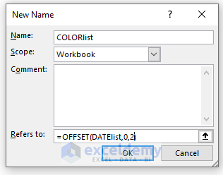
- Now, assign another name (i.e. COLORlist) for the column with header Color in the same way and assign the following formula:
=OFFSET(DATElist,0,2)Inside the formula,
- Datelist = Reference Range
- 0 = Rows to Offset
- 2 = Columns to Offset
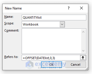
- However, Assign another name (i.e. QUANTITYlist) for the column with header Quantity in the same way and assign the following formula:
=OFFSET(DATElist,0,3)Here,
- DATElist = Reference Range
- 0 = Rows to Offset
- 3 = Columns to Offset
So, these are the two ways you can make the range dynamic. You can choose any of the above processes.
Date Range Selection and Chart Creating
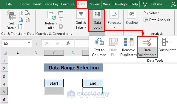
- Now assign the text Start & End to two cells in a new worksheet. Select the down cells of these two cells> go to the Data tab> click Data Validation.
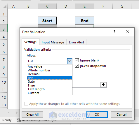
- After that, a Data Validation dialogue box will show up. Select List from Allow icon
- Now, assign the source by pressing the F3 key & the name list will show up. Select Datelist. You can also assign the source just by typing ‘Datelist’ (Your List name).

- Make sure to put a “=” sign before assigning the source in the box.

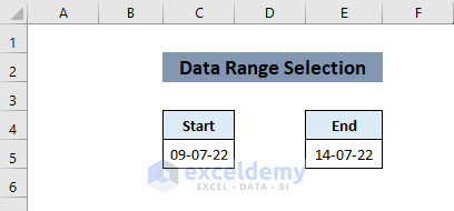
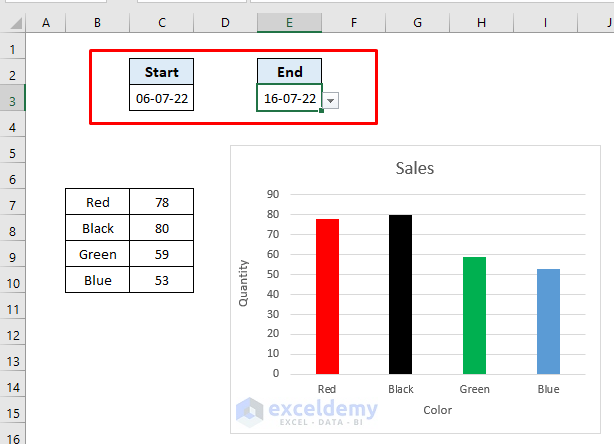
- Now both the selected cell will have a dropdown list. Click it and you will find the list of dates from the previous worksheet. Select a date.

- Pick a date for the cell. The down cell has the same date list.

- Select another date for the cell also.
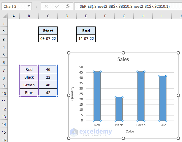
- The data we have used has four colors altogether: Red, Black, Green, and Blue. Assign these names to the cells where you want to get the result for these colors.

- Apply the following formula to the cell just right the first cell you have created just now (i.e. Red):
=SUMIFS(QUANTITYlist,DATElist,”>=”&$C$3,DATElist,”<=”&$E$3,COLORlist,B7)
Here,
- C3= Value of Start date
- E3= Value of End Date
- B7= Red (color)
- Now click ENTER and the value for the selected color and assigned date will be got. Use Autofill to drag the formula to the next cells. The result for all the colors will be ready.

- Now, create a column chart using the results. Click on any of the columns in the chart and all the columns will be selected.

- Then click again and now just one column will be selected. Right-click and the format box will show up. Change the color of the column as per the given name.
- Change the color of each column in this way.

- The result will change if you change the date from the dropdown option of the Start and End cell.
In this way, you can make the chart dynamic with the date range. The chart will show the relevant results by changing the dates.
Read More: How to Create Dynamic Chart with Multiple Series in Excel
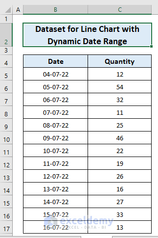
2. Line Chart with Dynamic Date Range
Let’s say, we have got a dataset for a quantity of different items in a shop over a certain period of time.
To create a line chart with a dynamic date range by using this method, just follow the steps below:
- At first, select any of the cells, go to the Insert tab and click Line Chart > choose a format.(i.e. 2D line)

- A line chart will be created.

- Then, select two cells, go to the Data tab> click Data Validation and two dropdown cells will be created just like the previous method.

- Now, create another two cells describing Date and Quantity. Apply the following formula (a combination of the INDEX and MATCH functions) to the cell just down the cell describing Date:
=INDEX($B$3:$B$15,MATCH($F$4,$B$3:$B$15,0)):INDEX($B$3:$B$15,MATCH($F$5,$B$3:$B$15,0))Inside the formula here,
- $B$3:$B$15= Data Range and lookup array
- $F$4= Start Date (dropdown cell)
- $F$5= End Date (dropdown cell)
- The MATCH function returns the position where it finds the match, the exact match since using 0, and then the INDEX function returns the value corresponding to the position from the range.

- Press ENTER and the result will show up. It may show either all the referred date cells or just the start date depending upon the version of Microsoft Excel.

- Apply the following formula to the next cell (i.e. Down cell of Quantity) and press ENTER.
=INDEX($C$3:$C$15,MATCH($F$4,$B$3:$B$15,0)):INDEX($C$3:$C$15,MATCH($F$5,$B$3:$B$15,0))Here,
- $B$3:$B$15= Data Range
- $B$3:$B$15= Lookup array
- $F$4= Start Date (dropdown cell)
- $F$5= End Date (dropdown cell)

- Now select the newly created cell (i.e. down cell of Date cell)> copy the formula applied to the cell. Go to the Formulas tab> click Name Manager.

- Now, the Name Manager dialogue box will show up. Click New.

- Assign a name to the Name box (i.e. DATEs) and paste the copied formula to the Refers to box and click OK.

- A new list will be created. Close the dialogue box.

- Select another created cell ( i.e. down cell of the Quantity cell) and repeat the same for this cell. Assign a name (i.e. QUANTITYs).

- QUANTITYs list will be created. Close the box.

- After that, right-click the chart> click Select Data.

- Click Edit on the Horizontal Axis Labels:

- Type the Sheet Name in the Axis label range box.

- Press F3 and the name list will show up. Select the list (i.e. DATEs) and click OK.

- You can also just type the list name (i.e. DATEs) in the Axis label range box. Then click OK.

- Now, click OK on the Select Data Source dialogue box.

- Finally, your chart will show a dynamic result.

- Change the date range in the Start and the End dropdown cell and you will see the change in the chart.
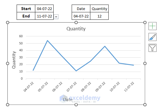
This is the way you can create a dynamic line chart in Excel.
Read More: How to Create Dynamic Charts in Excel Using Data Filters
Download Practice Workbook
Conclusion
In this article, we have learned how to create a chart with a dynamic date range in an Excel worksheet. I hope from now on, you can easily make a chart dynamic with the input dates in Excel. If you have any queries regarding this article, please don’t forget to leave a comment below. Have a great day!
Related Articles
- How to Make Dynamic Charts in Excel
- Create a Dynamic Chart Range in Excel
- How to Dynamically Change Excel Chart Data
- How to Create Dynamic Excel Charts with Drop-Down List
- How to Create a Dynamic Chart in Excel Using VBA
- How to Create Min Max and Average Chart in Excel
<< Go Back to Dynamic Excel Charts | Excel Charts | Learn Excel
Get FREE Advanced Excel Exercises with Solutions!
