How to Dynamically Change Excel Chart Data (3 Methods)

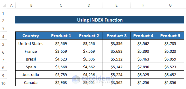
Method 1 – Using the INDEX Function

• In this method, we’ll create a dynamic chart in Excel that allows us to preview product sales amounts for various countries.
• We’ll use the INDEX function to achieve this dynamic behavior.

Steps

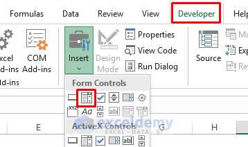
• Go to the Developer tab in the ribbon.
• From the Controls group, select the Insert drop-down option.
• Choose Combo Box from the Form Controls section.

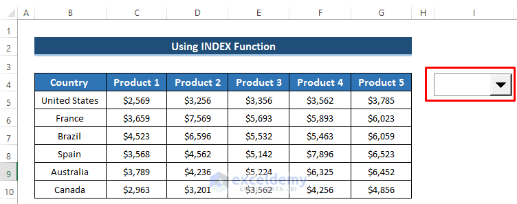
• Draw a box in any cell; it will look like the one shown in the screenshot.

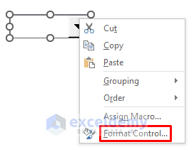
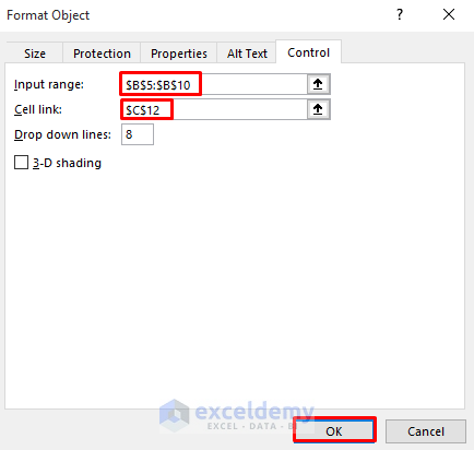
• Right-click on the combo box and select Format Control.

• In the Format Object dialog box, specify the input range (countries) for the chart.
• Select a cell link; it will change based on the combo box selection.
• Click OK.

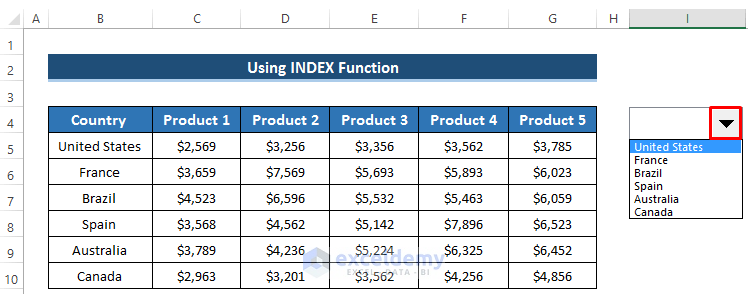
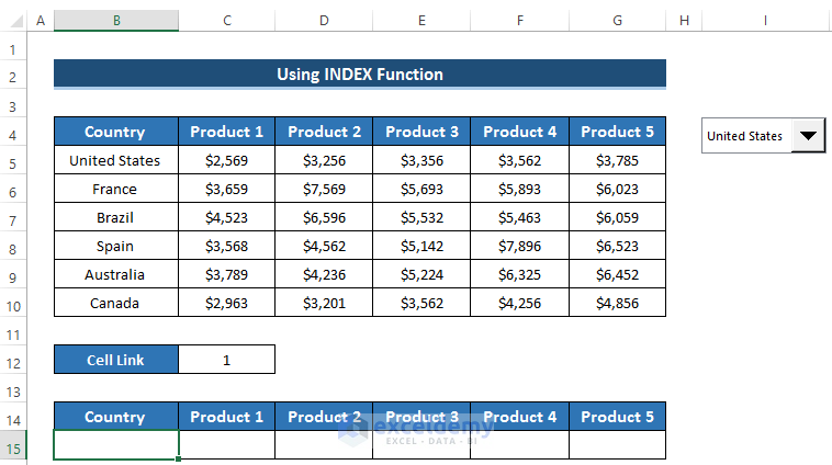
• Click the drop-down arrow on the combo box:
• You’ll see a list of country names from your dataset.

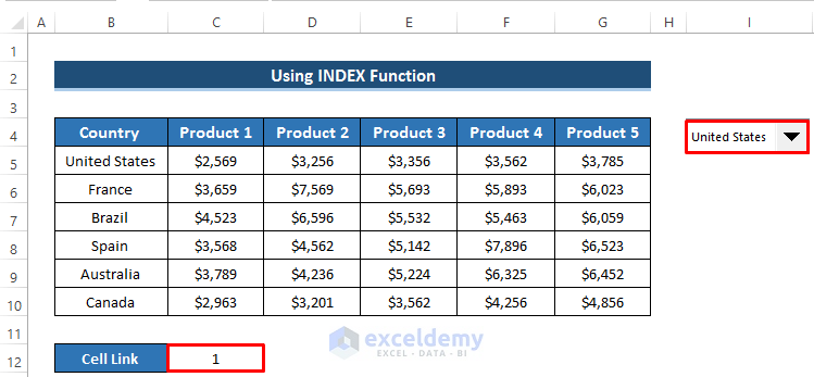
• The cell link will update accordingly. For example, selecting United States will show 1 as the cell link, while France will show 2.

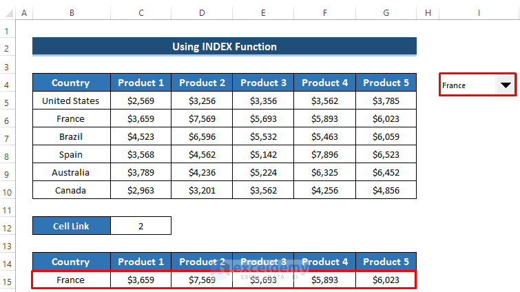
• Utilize the cell link and the INDEX function to create a dynamic Excel chart:
• Create headers for the dynamic chart.

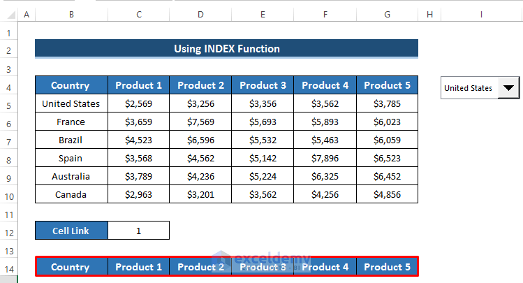
• Select cell B15.

• Enter the following formula in the formula box:

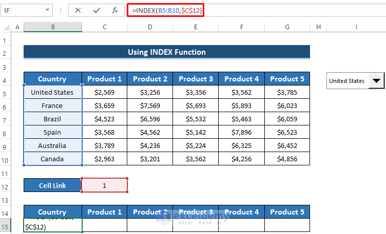
• Press Enter to apply the formula.

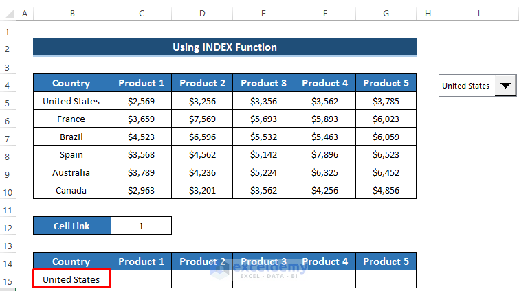
• Drag the Fill Handle icon right up to cell G15.

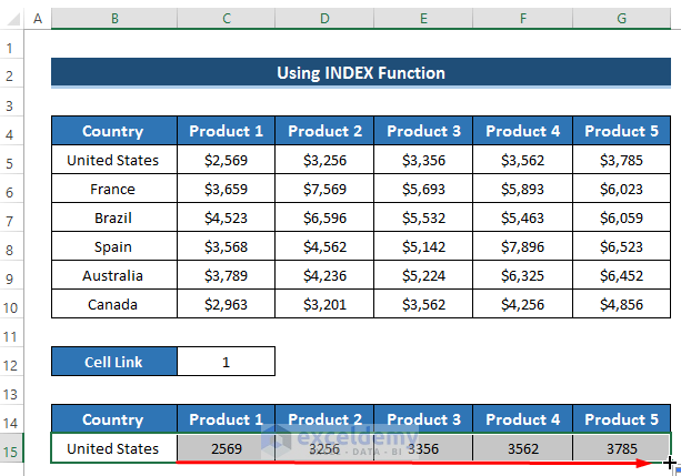
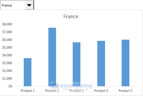
• Change the country from the drop-down option and select France.
• Observe how the dynamic table updates, shifting to France and displaying corresponding product sales amounts.

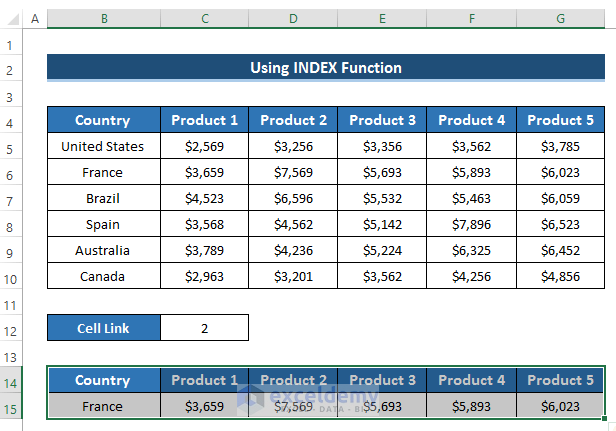
• Select the range of cells B14 to G15.

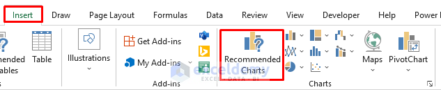
• Go to the Insert tab in the ribbon.
• From the Charts group, choose Recommended Charts.

• In the Insert Chart dialog box, select Clustered Column.
• Click OK.

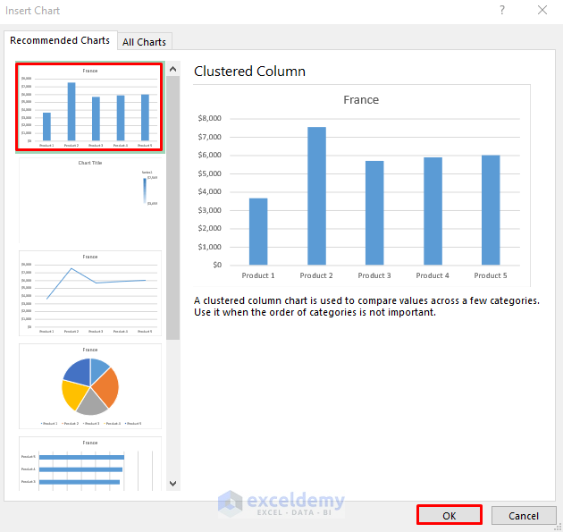
• You now have a dynamic chart representing the selected country.

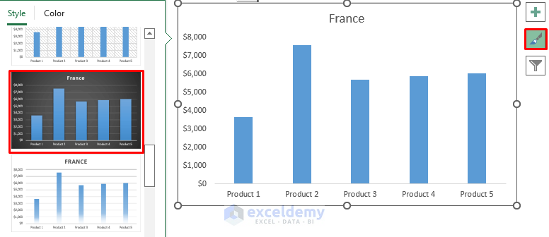
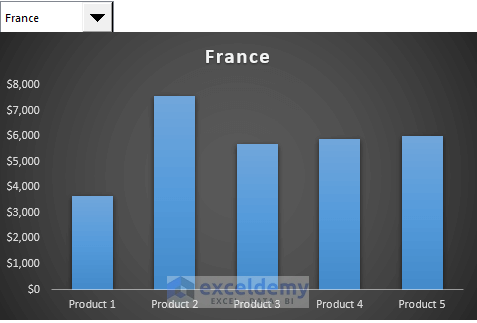
• Customize the chart style by clicking the brush icon and choosing your preferred style.

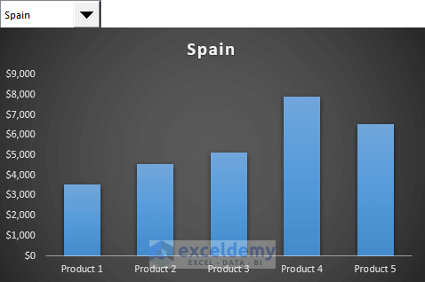
• The dynamic chart allows you to switch countries using the combo box:

• For example, select Spain to see the chart update accordingly.

Read More: How to Create Dynamic Excel Charts with Drop-Down List

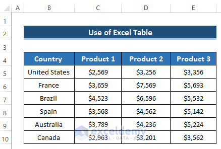
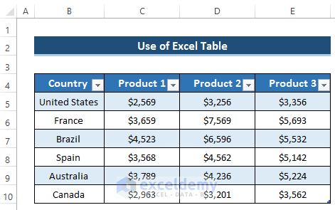
Method 2 – Using Excel Tables

• In this method, we’ll leverage Excel tables to create a dynamic chart.
• By adding or modifying data in the table, the chart will automatically update.

Steps

• Select the range of cells B4 to E10.

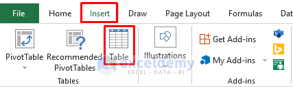
• Go to the Insert tab in the ribbon.
• From the Tables group, choose the Table option.

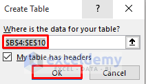
• The Create Table dialog box will appear.
• Select the range of cells.
• Click OK.

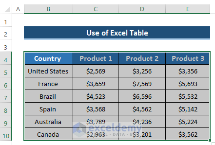
• Your dataset is now converted into a table.

• Select any cell in the table.
• Go to the Insert tab in the ribbon.
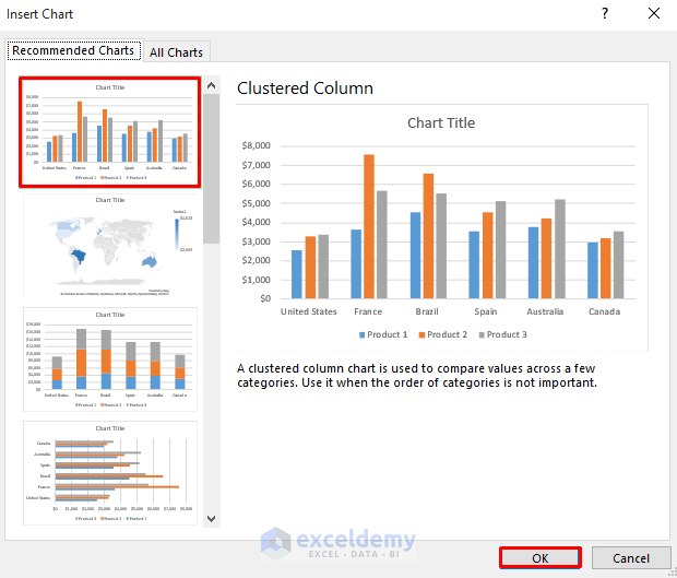
• From the Charts group, select Recommended Charts option.

• In the Insert Chart dialog box, choose Clustered Column.
• Click OK.

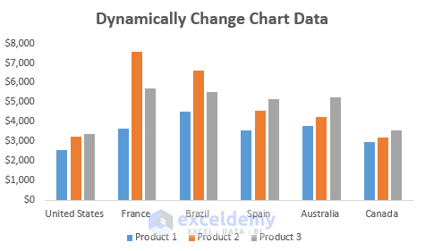
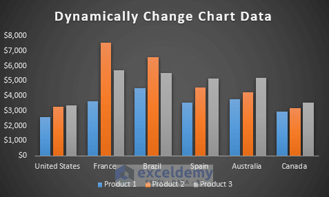
• You’ll have a dynamic chart that reflects changes in the table.

• Click the brush icon to modify the chart style.
• Select your preferred style.

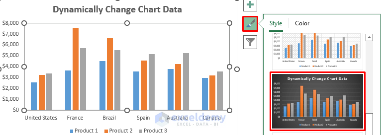
• The screenshot shows the result.

• As you add or modify data in the table (e.g., include a new country like China), the dynamic chart will update automatically.

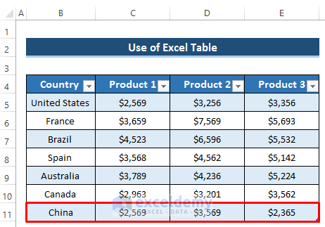
• Look at the dynamic chart, new data will be updated at the same time it is entered in the table.

Read More: How to Create Dynamic Charts in Excel Using Data Filters

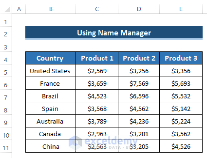
Method 3 – Using Name Manager for Dynamic Charts

• In this method, we’ll utilize the Name Manager feature in Excel to create a dynamic chart.
• By defining specific names for each column in our dataset, we can easily update the chart as data changes.

Steps

• Create dynamic named ranges using the OFFSET and COUNTA functions:
  • We have four columns in our dataset (Country, Product1, Product2, and Product3).
  • Follow these steps:
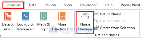
    • Go to the Formulas tab in the ribbon.
    • From the Defined Names group, select Name Manager.

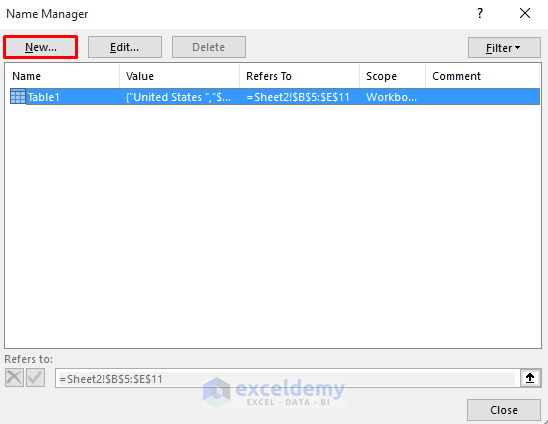
• • • Click New.

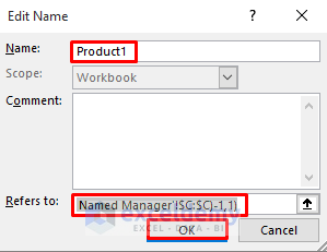
• • Set a preferred name (e.g., “Product1Range”) in the Name section.
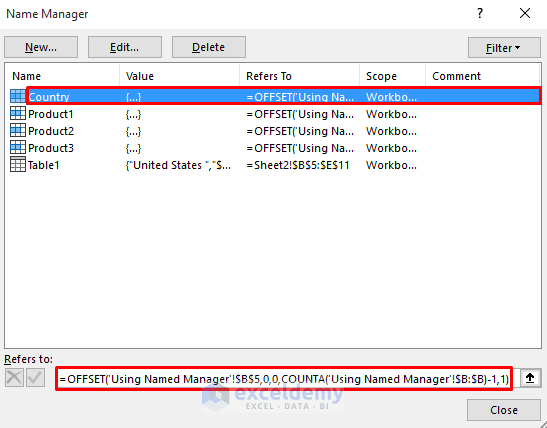
  • In the Refers to section, enter the following formula:

• • Click OK.

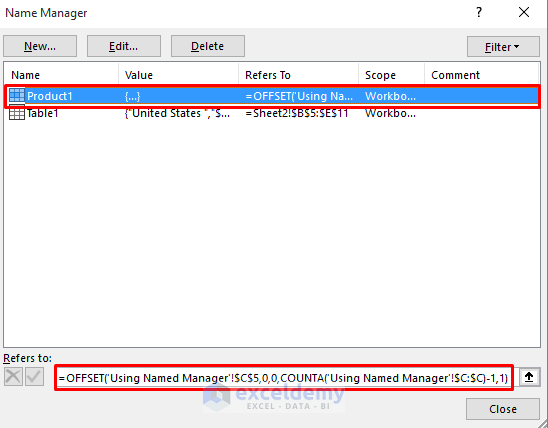
• • It will appear in the Name Manager dialog box.

• • Repeat the process for Product2, Product3, and Country.

• •  Create the dynamic chart:
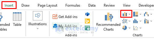
    • Go to the Insert tab in the ribbon.
    • From the Charts group, select Column Chart.

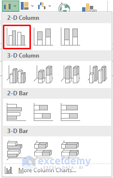
• • • Choose the first 2-D Column chart option (a blank sheet will appear).

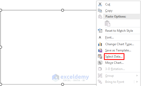
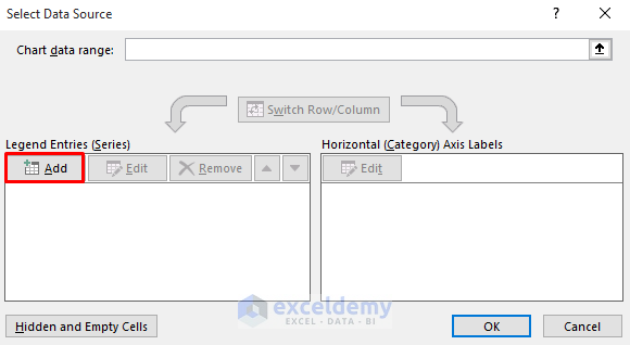
• • • Right-click on the chart and select Select Data.

• • • In the Legend Entries (Series) section, click Add to create new series.

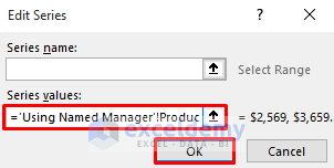
• • • For Series1, use the named range for Product1:

• • • Click OK.

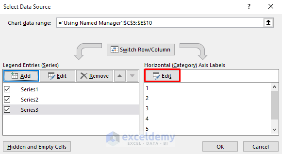
• • • It will create Series1 with the Product1 named range.
    • Repeat the process for Product2 and Product3 (Series2 and Series3).

• • • Edit the horizontal axis labels:
      • Use the Country named range for countries’ names.
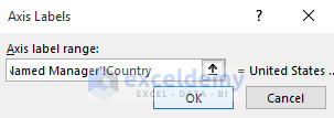
    • Enter the following in the Axis label range.

• • • Click OK.

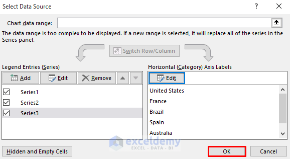
• • Finalize the dynamic chart:
    • Click OK in the Select Data Source dialog box.

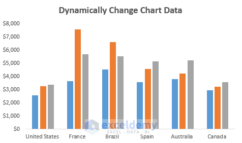
• • The resulting chart is dynamic:
    • As you modify data in your dataset (add, exclude, or update), the chart will automatically reflect those changes.

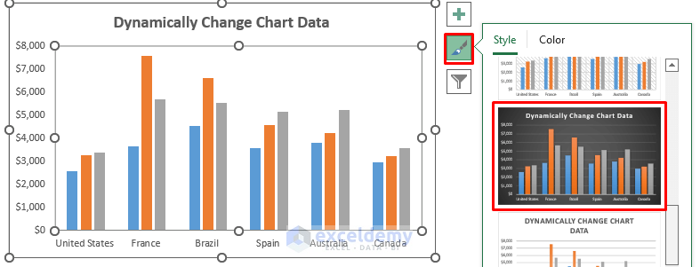
• • Customize the chart style by clicking the brush icon on the right side of the chart.
    • Select any of your preferences.

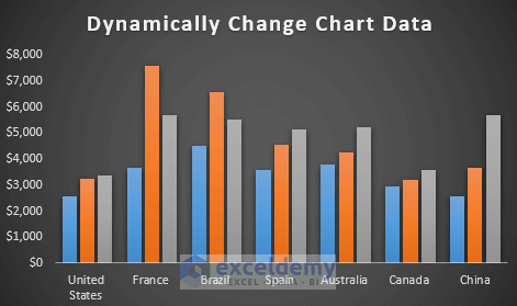
• • This is our final modified version of the dynamic chart. See the screenshot.

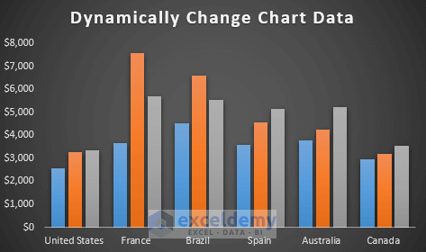
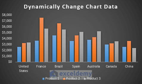
• • As it is a dynamic chart, if you change any data in your dataset or include or exclude any data, it will be updated in the dynamic chart automatically.
    • Now, include a new country China and their product sales amounts in your previous dataset.

• • • The dynamic chart will reflect the new data at the same time you enter it in the table.

Read More: How to Create Dynamic Chart with Multiple Series in Excel

Things to Remember

Worksheet Name:

• When defining named ranges, make sure to include the worksheet name along with it. This ensures that the named range refers to the correct data within the specified sheet.

Caution with OFFSET Function:

• Be cautious when using the OFFSET function in your named range formula.
• The OFFSET function returns a range based on a specified number of rows and columns from a starting point. Ensure that the parameters (such as row and column offsets) are correctly set to capture the desired data.

Handling INDEX Function Cell Link:

• If you’re using the INDEX function, pay attention to the cell link.
• The cell link should update dynamically based on user selections (e.g., country names in your case). Make sure it corresponds correctly to the chosen option in your combo box or other input controls.

Download the Practice Workbook

You can download the practice workbook from here:

Related Articles

• How to Create Chart with Dynamic Date Range in Excel
• How to Create a Dynamic Chart in Excel Using VBA 
• How to Create Min Max and Average Chart in Excel
• How to Make Dynamic Charts in Excel
• Create a Dynamic Chart Range in Excel

<< Go Back to Dynamic Excel Charts | Excel Charts | Learn Excel