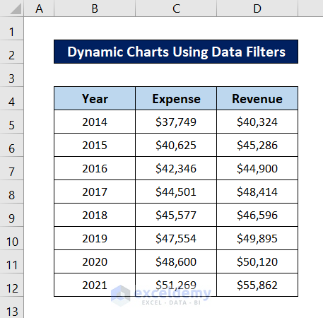
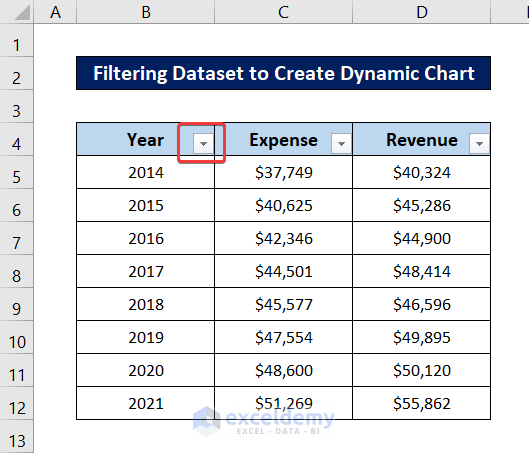
The following dataset will be used to create dynamic charts in Excel using data filters.
Method 1 – Filtering the Dataset to Create Dynamic Charts
Steps:
- Select the whole dataset (B4:D12).
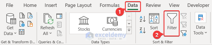
- Go to the Data tab.
- In Sort & Filter, select Filter.
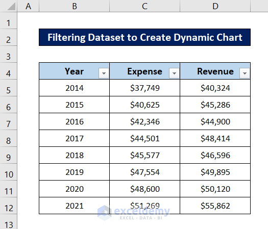
The dataset headers will display filters.
- Select the dataset again.
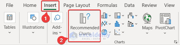
- Go to the Insert tab.
- In Charts, select Recommended Charts.
- The Insert Chart box will open.
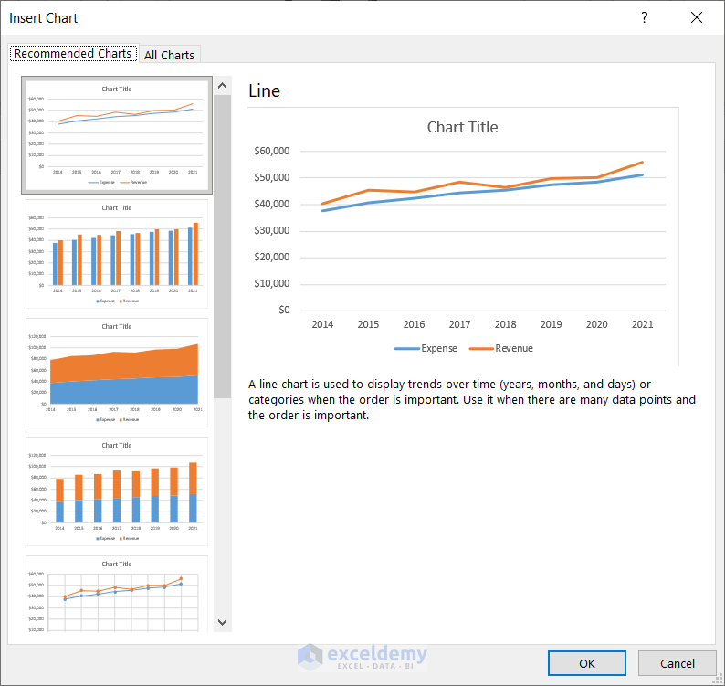
- Select a chart for the dataset. Here, the clustered column chart.
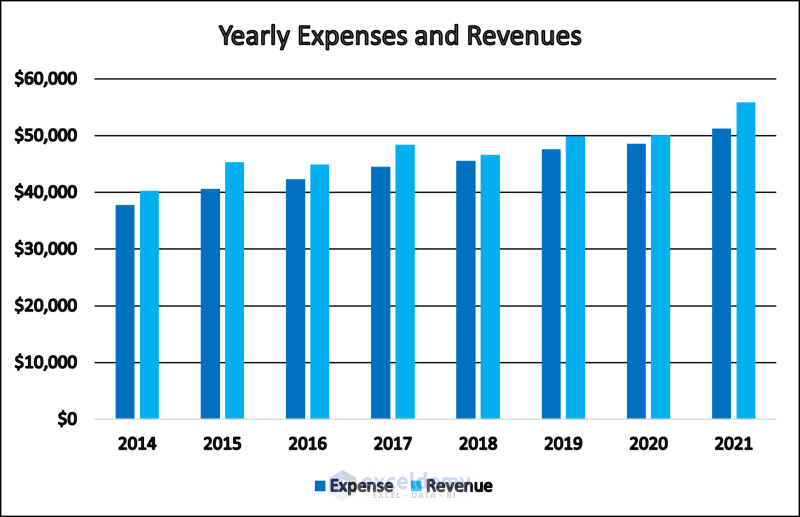
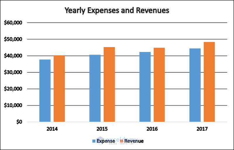
- Click OK and the chart will be displayed.
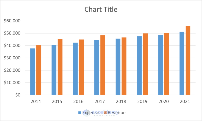
- Modify the graph.
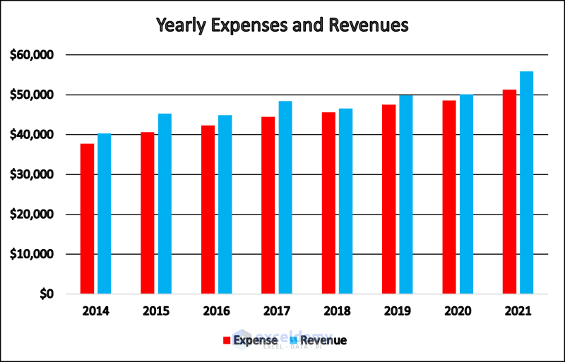
This chart can be used as a dynamic chart.
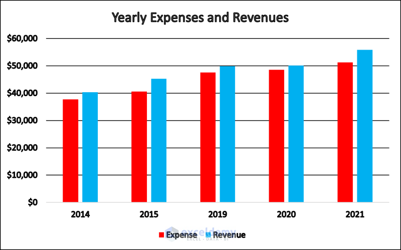
- Click the filter button in B4.
- Uncheck years 2016-2018. Click OK.
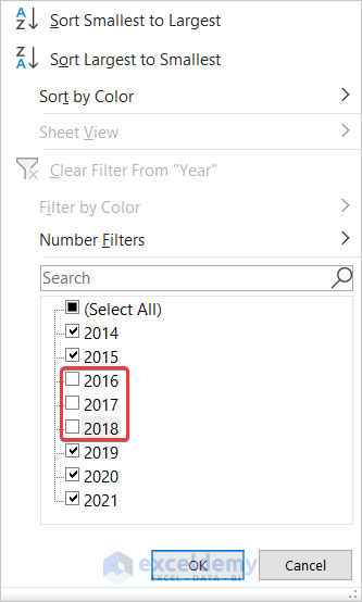
The graph will automatically change.
Read More: How to Create Dynamic Chart with Multiple Series in Excel
Method 2 – Using Chart Filters
Steps:
- Create a chart by selecting the whole dataset and choosing Recommended Charts from the Charts group in the Insert tab.
- Select a type of chart in Insert Chart. Here, the clustered column graph.
- Click OK and the chart will be displayed.
- Click the chart. Three additional features will be displayed.
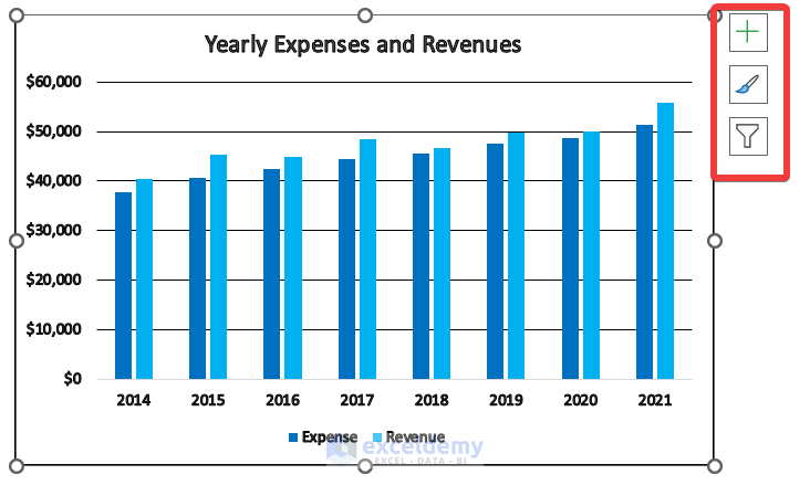
- Click Chart Filters to see the available filtering options.
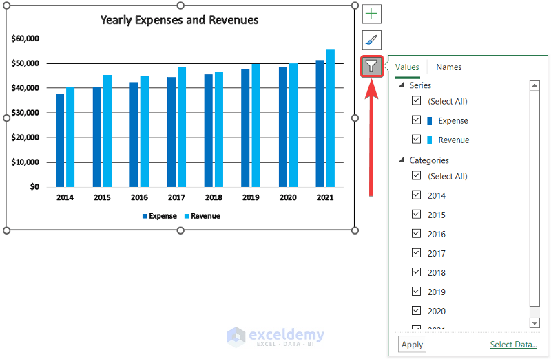
- You can modify your parameters. Here, “Revenue” and the years 2014-2017 were unchecked.
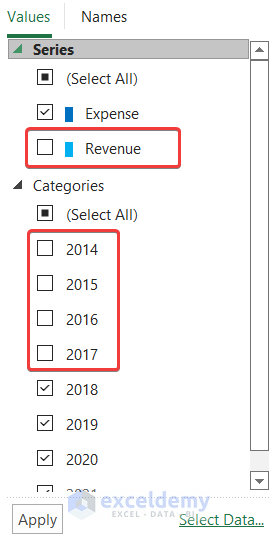
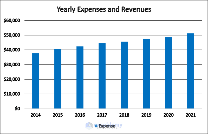
- Click Apply. Your graph will change.
Read More: How to Create Chart with Dynamic Date Range in Excel
Method 3 – Utilizing an Excel Table
Steps:
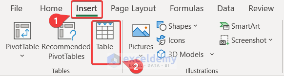
- Select the dataset or a cell in the dataset.
- Go to the Insert tab.
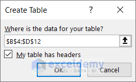
- In Tables, select Table.
- Click OK in Create Table. Make sure that My table has headers is checked.
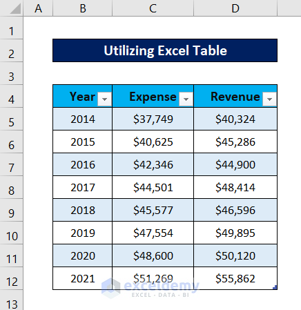
The dataset is converted to an Excel table.
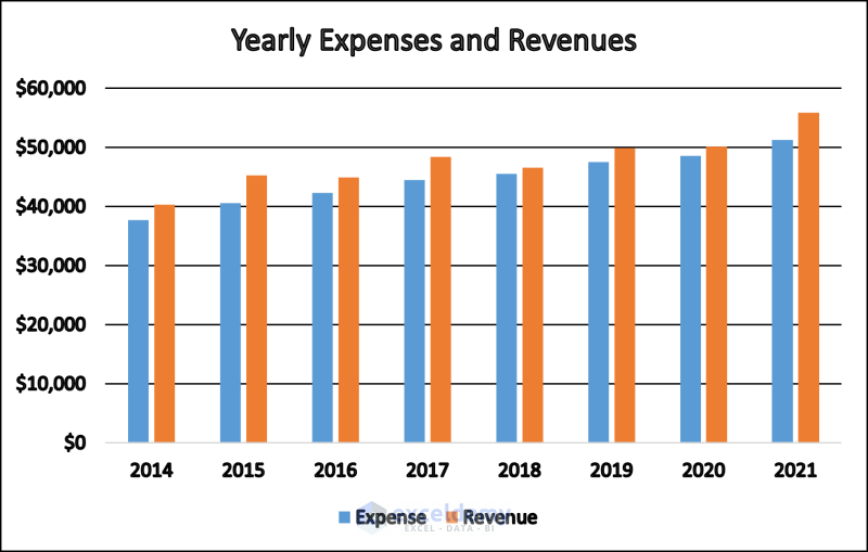
- Create a chart by selecting the whole dataset and choosing Recommended Charts from the Charts group in the Insert tab.
- Select a type of chart in Insert Chart. Here, the clustered column graph.
- Click OK and the chart will be displayed.
- Use the data filters in the table headers to change the chart parameters. For example, click the filter in B4.
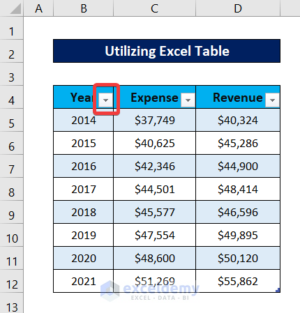
- Select your parameters. Years 2018-2021 were unchecked.
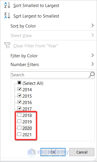
- Click OK and the chart will automatically change.
Read More: How to Create a Dynamic Chart in Excel Using VBA
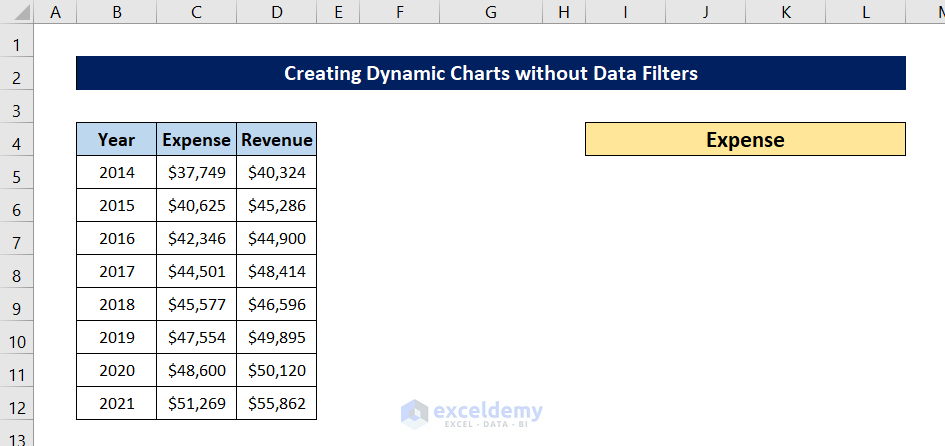
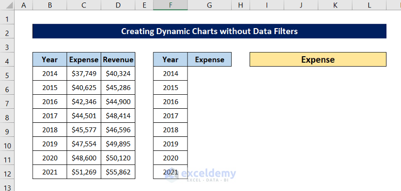
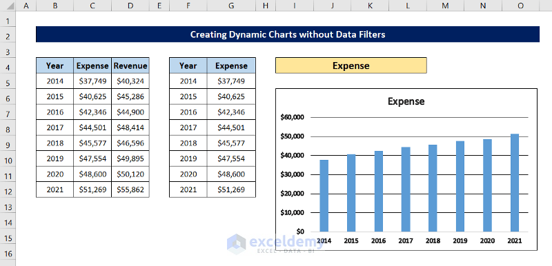
How to Create Dynamic Charts Without Data Filters in Excel
Steps:
- Select I4.
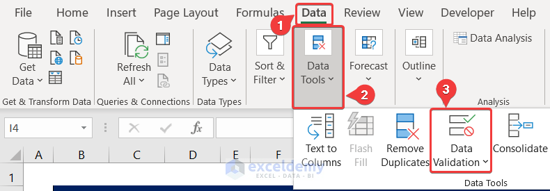
- Go to the Data tab.
- In Data Tools, select Data Validation.
- In the Data Validation window, select Settings.
- In Allow, select List.
- In Source, enter Expense, Revenue.
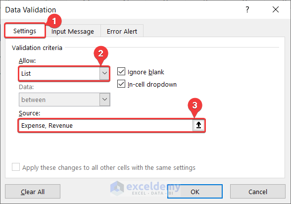
- Click OK.
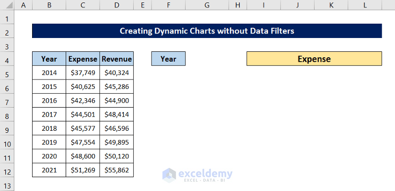
A data filter will be created in the cell.
- Create a header for the years in F4.
- Select G4 and enter the following formula.
=I4
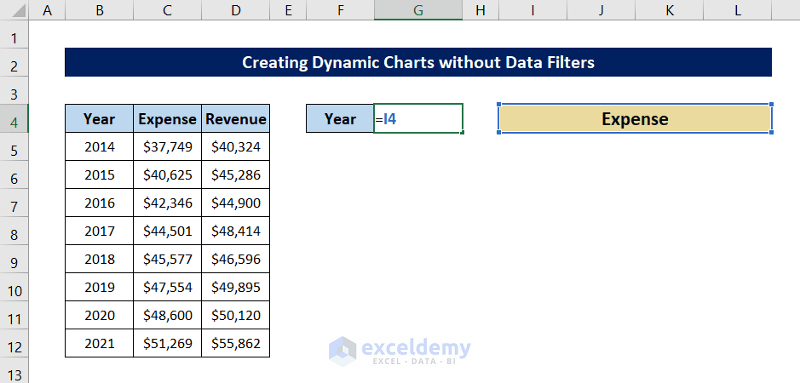
- Press Enter.
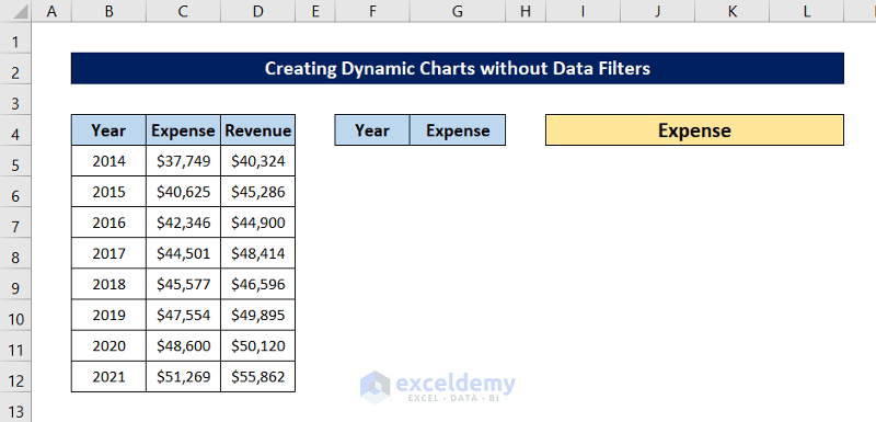
- Copy all years to F5:F12.
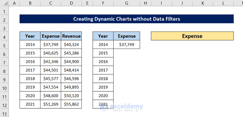
- Select G5 and enter the following formula.
=INDEX($C$5:$D$12,MATCH(F5,$B$5:$B$12,0),MATCH($G$4,$C$4:$D$4,0))
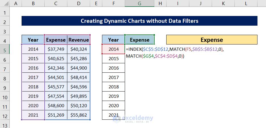
- Press Enter.
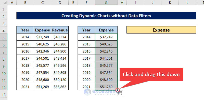
- Select the cell again and drag down the fill handle to fill the rest of the cells with the formula.
- Select F4:G12 and go to the Insert tab.
- In Charts, select Recommended Charts.
- Select a chart in Insert Chart. Here, the column chart.
- Click OK and the chart will be displayed.
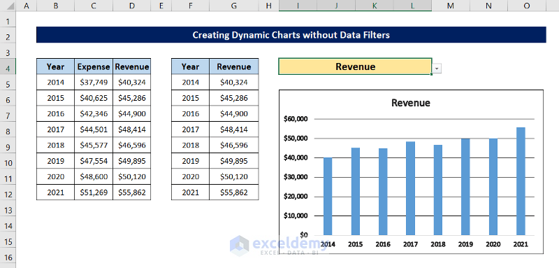
- Select I4 and change the option to Revenue.
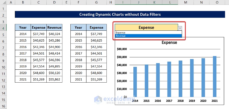
The chart will automatically change.
Download Practice Workbook
Related Articles
- How to Make Dynamic Charts in Excel
- Create a Dynamic Chart Range in Excel
- How to Create Min Max and Average Chart in Excel
- How to Dynamically Change Excel Chart Data
- How to Create Dynamic Excel Charts with Drop-Down List
<< Go Back to Dynamic Excel Charts | Excel Charts | Learn Excel
Get FREE Advanced Excel Exercises with Solutions!
