How to Create a Dynamic Chart in Excel Using VBA (5 Easy Steps)

Dataset Overview

We have a worksheet called Dataset that contains a table with the Country, Revenue, and Earnings of a company.

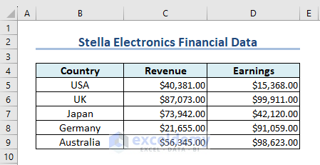
Our objective today is to generate a dynamic chart from this table using Excel VBA.

Step 1 – Creating an Excel Table

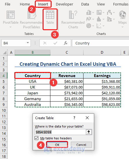
Open your workbook and navigate to the worksheet containing your data (in this case, the Dataset).
Select any cell within the dataset.
Go to the Insert tab and click on Table. Confirm by clicking OK.

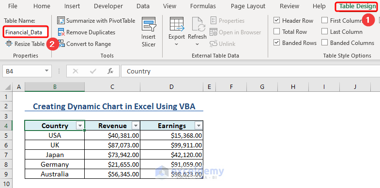
In the Table Design contextual tab, rename the table to Financial_Data.

Step 2 – Open the Visual Basic Window and Insert a New Module

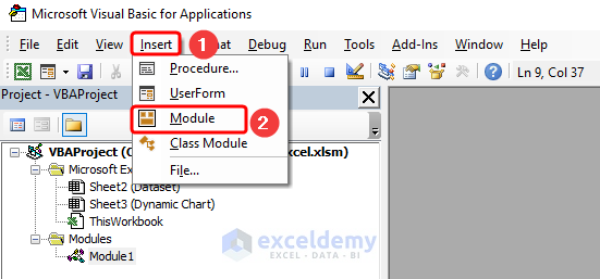
Press ALT + F11 on your keyboard to open the Visual Basic for Applications (VBA) window.
Go to Insert and select Module to insert a new module (let’s call it Module1).

Step 3 – Add the VBA Code

Paste the following VBA code inside the Module window:

Sub Create_Dynamic_Chart()

Dim wsht As Worksheet
Dim chrt As Chart
Dim data_rng As Range

Set wsht = ActiveSheet
Set data_rng = Range("Financial_Data")
Set chrt = wsht.Shapes.AddChart2(Style:=-1, Width:=600, Height:=400, _
Left:=Range("G1").Left, Top:=Range("G1").Top).Chart

With chrt

    .SetSourceData Source:=data_rng
    .ChartType = xlColumnClustered
    .chartTitle.Text = "Revenue and Earnings by Country"
    .SetElement msoElementDataLabelOutSideEnd
    .SetElement msoElementPrimaryValueGridLinesMajor
    .SetElement msoElementPrimaryValueAxisShow
    .SetElement msoElementLegendBottom
    .SetElement msoElementPrimaryCategoryAxisTitleBelowAxis
    .Axes(xlCategory).AxisTitle.Text = "Country"
    
    
End With

End Sub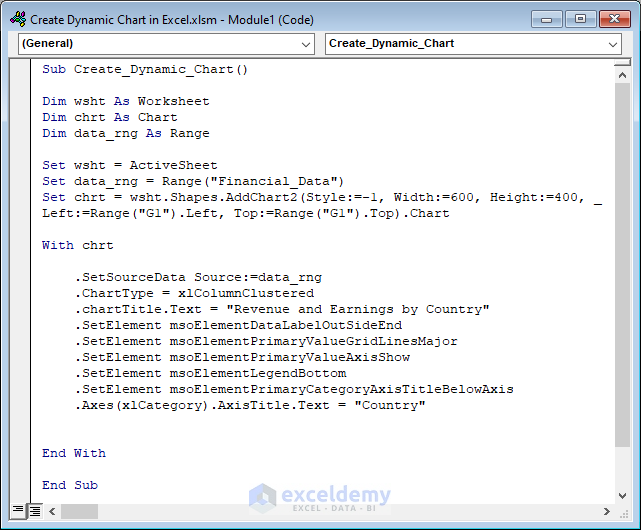

This code creates a dynamic chart based on the Financial_Data table.

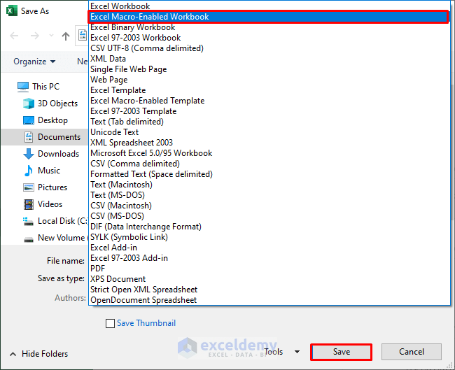
Step 4 – Save the Workbook in XLSM Format

Return to your workbook and save it as an Excel Macro-Enabled Workbook (XLSM).

Step 5 – Run the Macro

Click the Run button or press F5 to execute the macro.

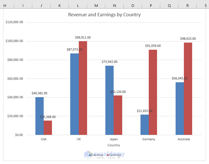
Your dynamic chart should now be generated!

Things to Remember

Remember that using a table is the best approach because it automatically adjusts when you add or remove data. However, you can also achieve this using a Named Range or other methods.