How to Create Dynamic Chart with Multiple Series in Excel

Fortunately, many of us use Excel in our business organizations. In any business organization, we use Excel to organize data as per need and make databases for the future. Moreover, one interesting thing is that we can create a dynamic chart with multiple series easily in Excel. However, I have used Microsoft Office 365 for the purpose of demonstration, and you can use other versions according to your preferences. In this article, I will show you 2 suitable methods to create a dynamic chart with multiple series in Excel. Hence, read through the article to learn more and save time.

How to Create Dynamic Chart with Multiple Series in Excel: 2 Suitable Methods

In this tutorial, I will show you how to create a dynamic chart with multiple series and the process becomes more interesting with Excel. However, the task is easy and simple. But you will need an arrangement in order to perform the operation properly. Usually, Dynamic Chart automatically updates itself when the data source gets updated. In contrast, the Static Chart does not update when the data source is changed. Here, I have used 2 different methods to make you understand the scenario properly. For the purpose of demonstration, I have used the following sample dataset.

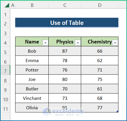
1. Insert Table to Create Dynamic Chart with Multiple Series

Fortunately, you can convert a set of data in an Excel spreadsheet into an Excel Table. Additionally, this Excel table can help create a dynamic chart range. However, the process is quite simple and easy. Hence, read through the steps below in order to complete the operation properly.

📌 Steps:

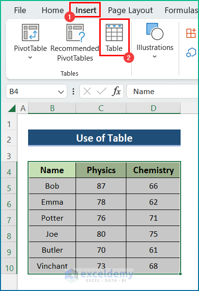
Initially, select the complete dataset.
Then, go to the Insert tab and select Table.

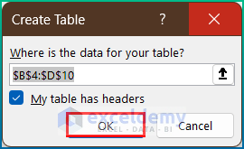
From the Create Table dialog box, press OK.

Next, the dataset will be converted into a table.
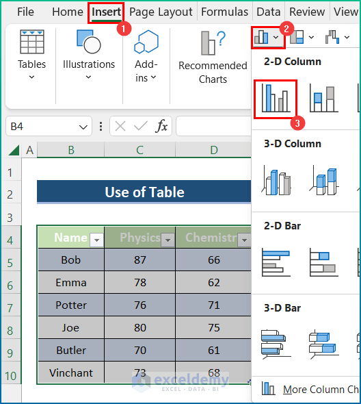
Now, select the table.
Similarly, move on to the Insert tab and select Insert → Charts → 2-D Column → Clustered Column.

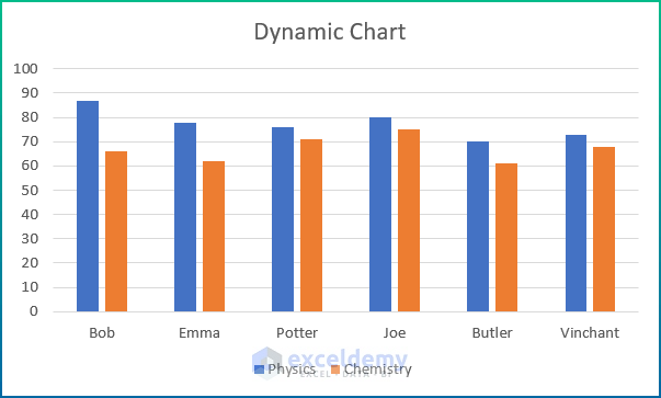
After that, a 2-D Column chart will appear and this is the Dynamic Chart.

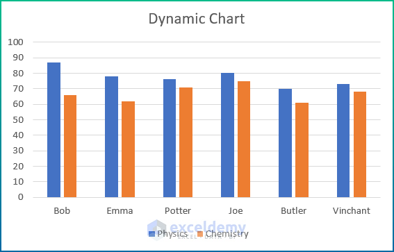
Now, I will add a new row to the table. Let’s say, I will add Olivia’s securing marks in Physics and Chemistry as 91 and 77.

Consequently, the chart with multiple series updates the data automatically.
As a result, we can say the chart is a dynamic one.

2. Create Dynamic Chart Through Named Range in Excel

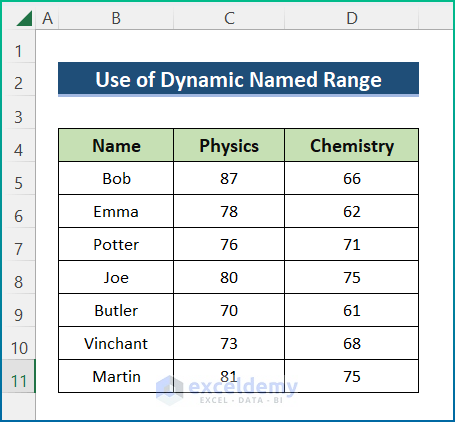
In general, the easiest way to create a dynamic chart range is to use Excel Table. But for some reason, if you can’t use the previous method, then you can combine the OFFSET and COUNTA functions to create a dynamic chart range in Excel. Here, I will use Dynamic Named Range to complete the task. However, the dynamic named range is a feature in Excel that adjusts the range automatically when we add or remove data to the range. Hence, go through the steps mentioned below.

STEP 1: Define Named Range

Firstly, I will make the defined name and the dynamic formula for every column.
For this purpose, in the Formulas tab, go to Defined Names → Defined Name.

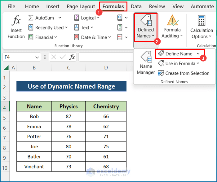
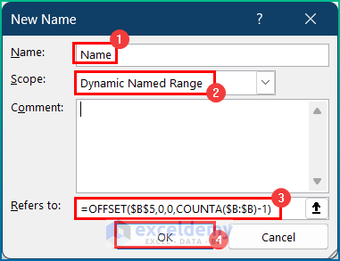
Hence, a New Name dialog box will appear in front of you. In that dialog box, type Name in the Name typing box.
Secondly, select the current worksheet named Dynamic Ranged Name from the Scope drop-down box.
Thirdly, type the below formulas in the Refers to typing box and press OK.

=OFFSET($B$5,0,0,COUNTA($B:$B)-1)

🔎 Formula Breakdown:

In the above formula, the COUNTA function counts all the non-empty cells from the entire column data of column B and here it returns 8.
Next, the OFFSET function returns a range of cells from the specified rows and columns.
Here, it takes the reference value as B5 and height as the output provided by the COUNTA function.
Finally, it returns the value of the non-empty cells of column B.

Similarly, repeat the above-described steps for column C. However, the formula for the Physics column will be as below.

=OFFSET($C$5,0,0,COUNTA($C:$C)-1)

Again, insert the below formula for the Chemistry column to perform a similar process.

=OFFSET($D$5,0,0,COUNTA($D:$D)-1)

STEP 2: Creating Dynamic Chart in Excel

Now, draw a 2-D Stacked Bar chart from the Insert tab following the similar process mentioned in the 1st Here, I have selected the full dataset B4:D10 for the chart.

After that, press right-click on any column of your chart. Instantly, the Context Menu pops up.
Now, select the Select Data option from that window.

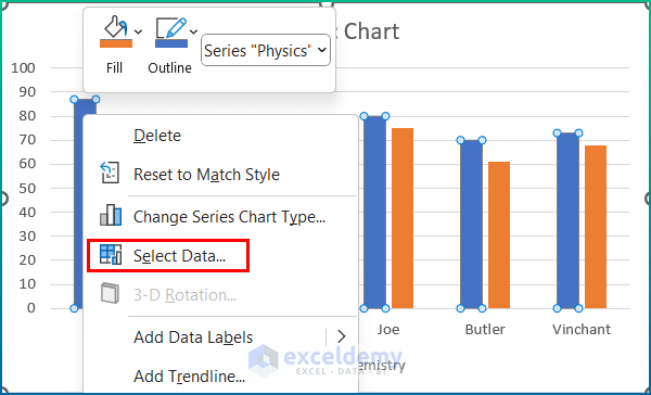
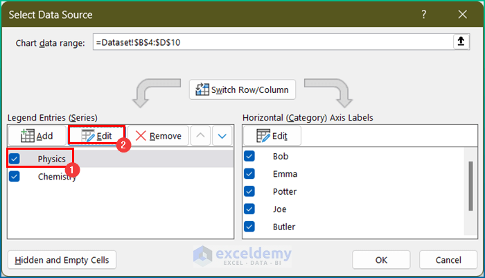
As a result, a Select Data Source dialog box will appear in front of you. From the Select Data Source dialog box, firstly, select Physics.
Secondly, select the Edit option under the Legend Entries (Series).

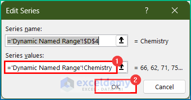
Consequently, a window named Edit Series pops up. From the Edit Series dialog box, type =’Dynamic Named Range’!Physics in the Series values typing box.
At last, press OK.

Similarly, from the Edit Series dialog box, type =’Dynamic Named Range’!Chemistry in the Series values typing box.
Again, press OK.

After that, select the Edit button under the Horizontal (Category) Axis Labels option.

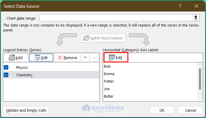
From the Axis Labels dialog box, type =’Dynamic Named Range’!Name in the Axis label range box and press OK.

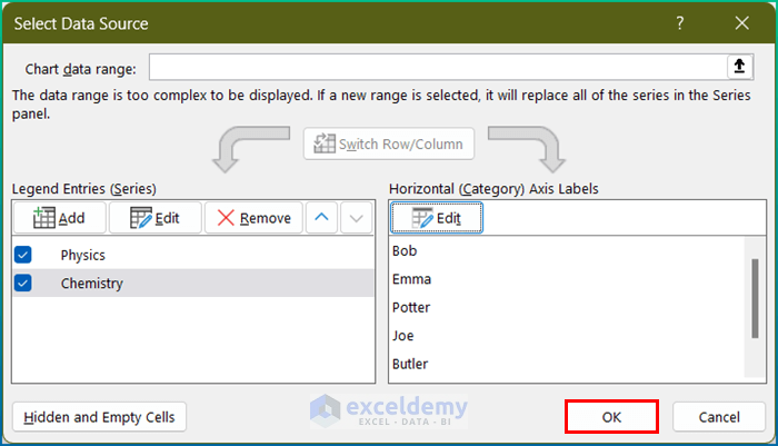
Again, press OK.

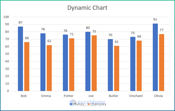
Final Output

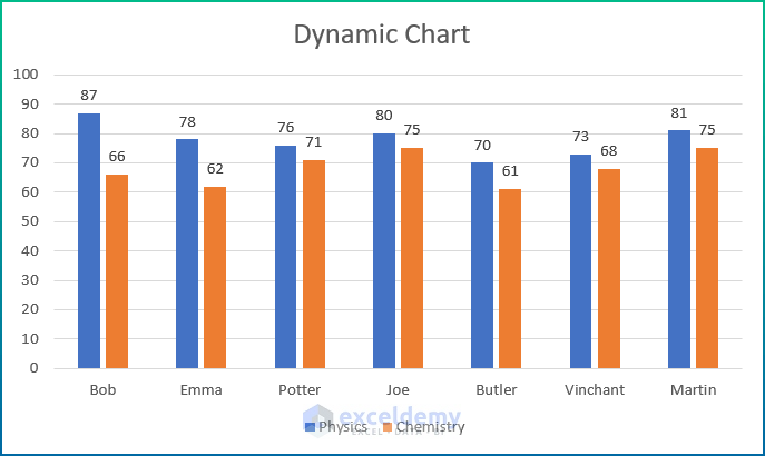
In the end, I will add a new row to the table. Let’s say, I will add Martin’s securing marks in Physics and Chemistry as 81 and 75.

Consequently, the chart with multiple series updates the data automatically.
Hence, see the below chart to understand clearly.

💬 Things to Remember

First of all, if there is no value in the referenced cell, the #N/A error occurs in Excel.
Then, you can press Ctrl + T simultaneously on your keyboard to create a table.
Next, you should not leave any blank cells in the Named Range.
Afterward, make sure to follow the naming convention when entering the Series values.

Download Practice Workbook

Dynamic Chart with Multiple Series.xlsx

Conclusion

These are all the methods you can follow to create a dynamic chart with multiple series in Excel. Overall, in terms of working with time, we need this for various purposes. I have shown multiple methods with their respective examples, but there can be many other iterations depending on numerous situations. Hopefully, you can now easily create the needed adjustments. I sincerely hope you learned something and enjoyed this guide. Please let us know in the comments section below if you have any queries or recommendations.

<< Go Back to Dynamic Excel Charts | Excel Charts | Learn Excel

Get FREE Advanced Excel Exercises with Solutions!