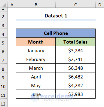
How to Create Dynamic Charts in Excel - 3 Methods

The dataset shows Month, and Total Sales in USD.

Method 1 – Creating Dynamic Charts Using an Excel Table

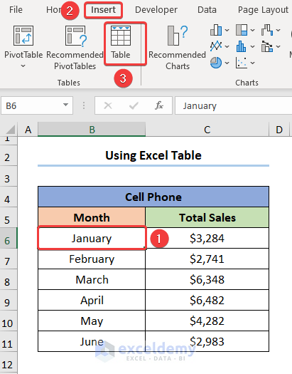
Steps:

Select any cell within the dataset.
Go to Insert > Table.

Select B5:C11 and check My table has headers.

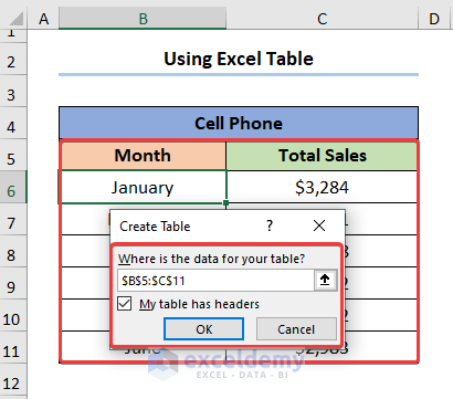
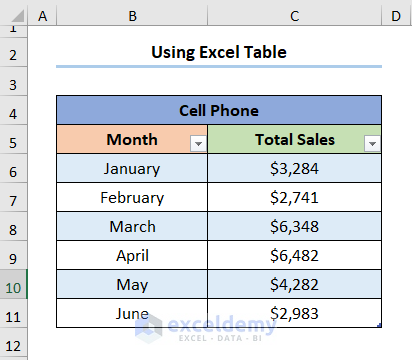
This is the output.

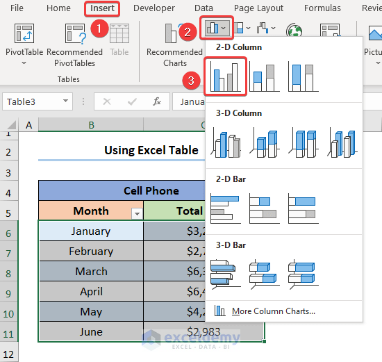
Select the dataset.
Go to Insert > Insert Column or Bar Chart > Clustered Column.

Customize your chart using the Chart Elements option.

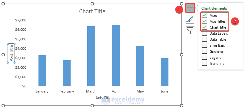
A Dynamic Chart is created.

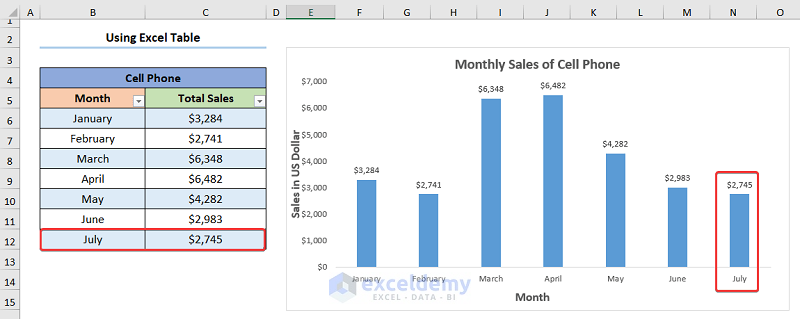
Add the Total Sales for July and the chart will automatically update.

Method 2 – Using a Dynamic Named Range with the OFFSET Function to Create Dynamic Charts

Step 1: Define the Named Range

Go to Formulas > Define Name.

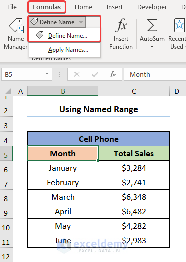
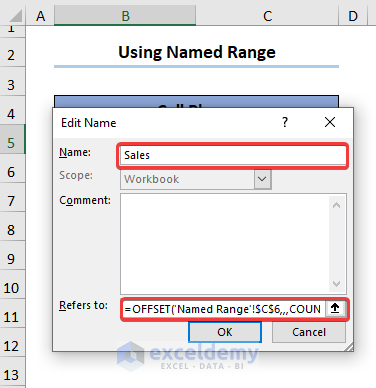
Click Define Name and name the data range.
Enter the formula in Refers to.

=OFFSET('Named Range'!$C$6,,,COUNTIF('Named Range'!$C$6:$C$100,"<>"))

C6 is the first cell in the Total Sales column.

⚡ Formula Breakdown:

The OFFSET function returns a range from the specified rows and columns.
The ‘Named Range’!$C$6 is the reference argument that provides the initial point of the range.
The rows and cols argument is left blank.
The COUNTIF(‘Named Range’!$C$6:$C$100,”<>”) is the optional height argument.
C6:C100 is included in the (range argument) to add rows to the data table.
The “<>” (criteria argument) returns the values of all non-blank cells.

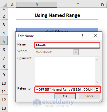
Create a second Named Range for the Month column using the expression below.

=OFFSET('Named Range'!$B$6,,,COUNTIF('Named Range'!$B$6:$B$100,"<>"))

B6 indicates the starting point of the Month column and again we select up to B100.

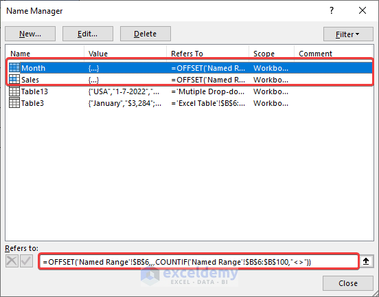
Go to Formulas > Name Manager:

You can see all Names.

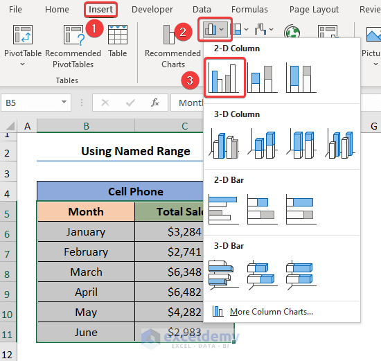
Step 2: Insert a Column Chart

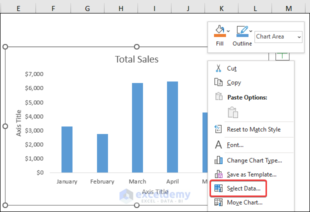
Go to Insert > Insert Column or Bar Chart > Clustered Column.

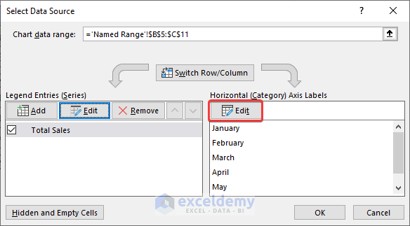
Select the chart and right-click to go to Select Data.

In the dialog box, click Edit.

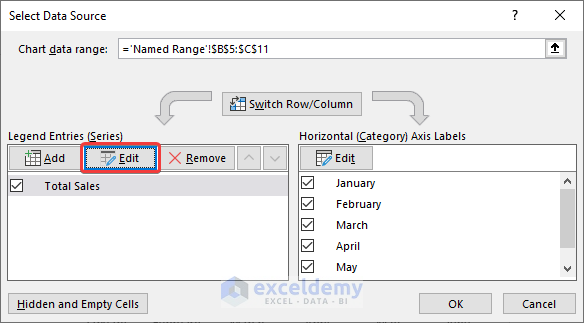
Select the cell reference and press F3.
In Names, choose Sales.

Click OK.

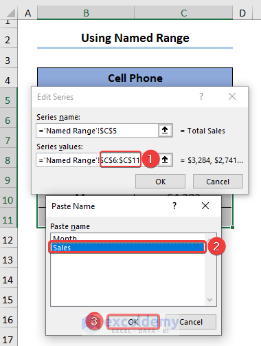
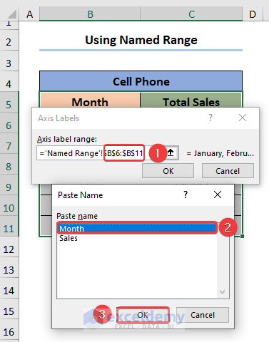
Click Edit to change the x-axis labels.

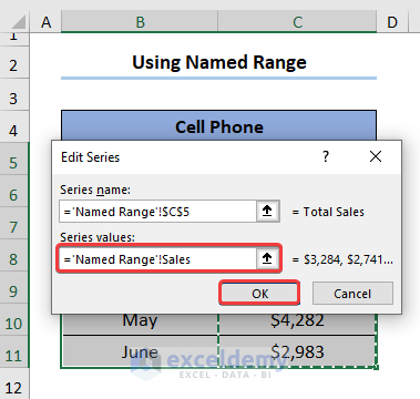
Change the Series value for Month as shown below.

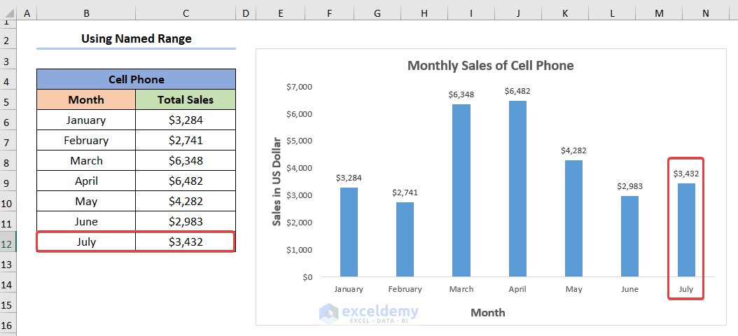
Add a row for July to check whether the chart updates automatically.

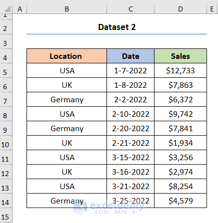
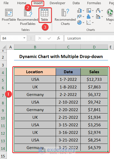
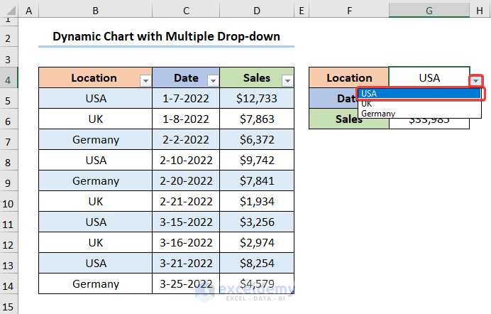
Method 3 – Creating Dynamic Charts with Multiple Drop-Downs in Excel

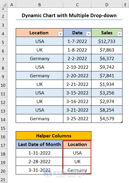
The dataset showcases Location, Date, and Total Sales in USD.

Step 1: Insert a Table and Helper Columns

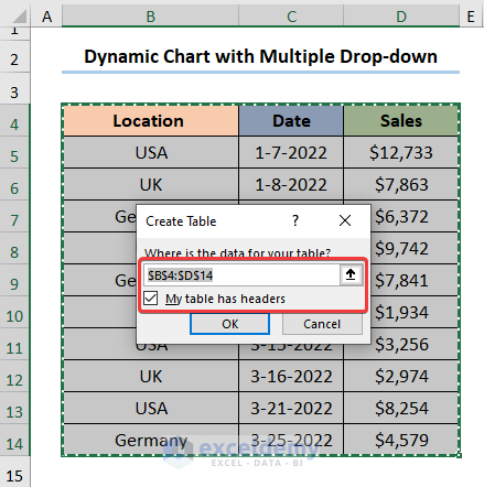
Select any cell in the dataset and go to Insert > Table.

Select B5:D14 and check My table has headers.

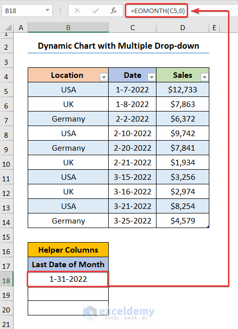
In B18, enter the formula.

=EOMONTH(C5,0)

C5 refers to the start date of the dataset.

The EOMONTH function returns the last day of the month using C5 (start_date argument) and 0 (months argument).

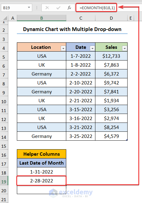
Use the formula below to get the last day of the second month.

=EOMONTH(B21,1)

B21 (start_date argument) points to the last day of the previous month. 1 (months argument) returns the last day of the next month.

Copy the names in Location and paste them in the column.

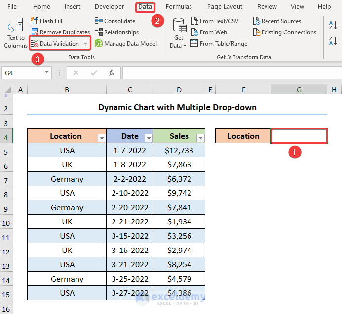
Step 2: Insert a Data Validation List

Select G4 and go to Data > Data Validation.

Choose List in Allow and select C19:C21 as Source.

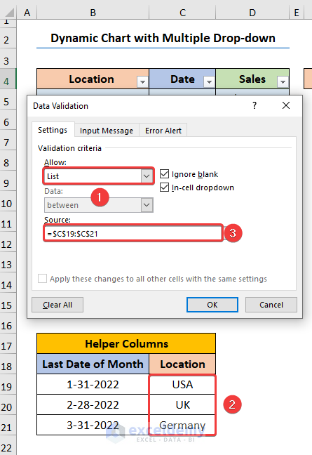
Follow the same steps for Date and choose B19:C21.
In Sales enter the expression below.

=SUMIFS($D:$D,$B:$B,G4,$C:$C,"<="&G5)

Formula Breakdown:

The SUMIFS function adds all cells that meet the multiple criteria.
$D:$D (sum_range argument) is added to Sales values.
$B:$B (criteria_range1 argument) refers to Locations.
G4 (criteria1 argument) indicates the criteria to apply to the Location column.
$C:$C (criteria_range2 argument) points to Date.
“<=”&G5 (criteria2 argument) is the criteria for choosing all Dates less than and equal to the value in G5.

Note: Provide Absolute Cell Reference ($) for columns B, C, and D.

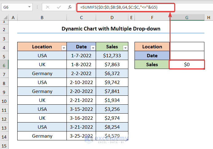
This is the output.

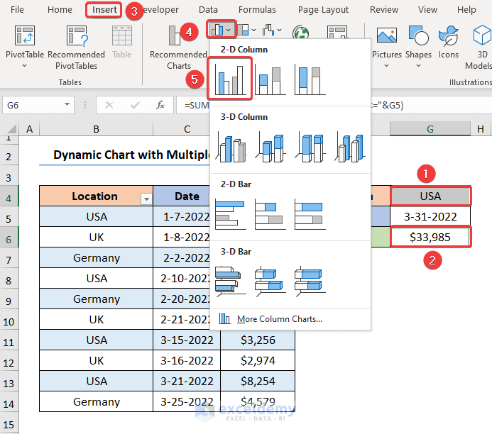
Step 3: Insert a Bar Chart

Select G4 and G5.
Go to Insert > Insert Column or Bar Chart > Clustered Column.

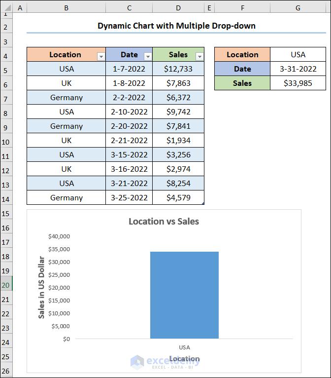
The Bar Chart is displayed.

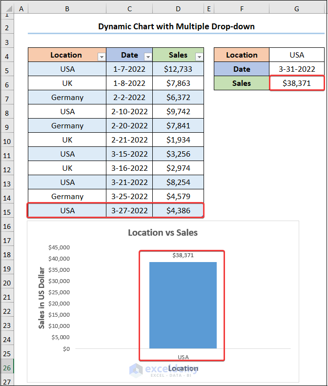
Add an entry for USA, and the Sales value will update.

Things to Remember

Don’t leave blank cells in the Named Range.
Follow the naming convention when entering the Series values. Enter the ‘Named Range’ (Sheet Name) within single quotes, followed by an Exclamation (!) sign, and Sales (Defined Name).