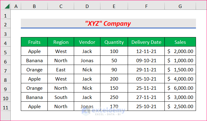
The sample dataset showcases Fruits, Region, Vendor, Quantity, Delivery Date and Sales.
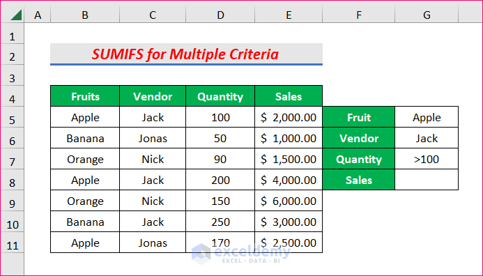
You want to sum Sales or Quantity values based on different criteria.
Method 1: Using the SUMIFS function for Multiple Criteria with a Comparison Operator
Step 1:
- The output cell is G8
- Enter the following formula in G8.
=SUMIFS(E5:E11,B5:B11,G5,C5:C11,G6,D5:D11,">"&100)E5:E11 is the sum range
And B5:B11, C5:C11, and D5:D11 is the criteria range
G5, G6, and “>”&100 are the criteria.
If all criteria are met, sales values will be summed.
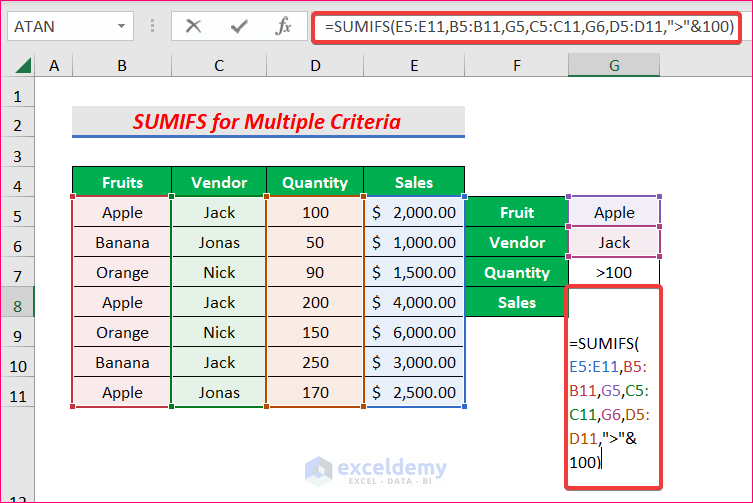
- Press ENTER.
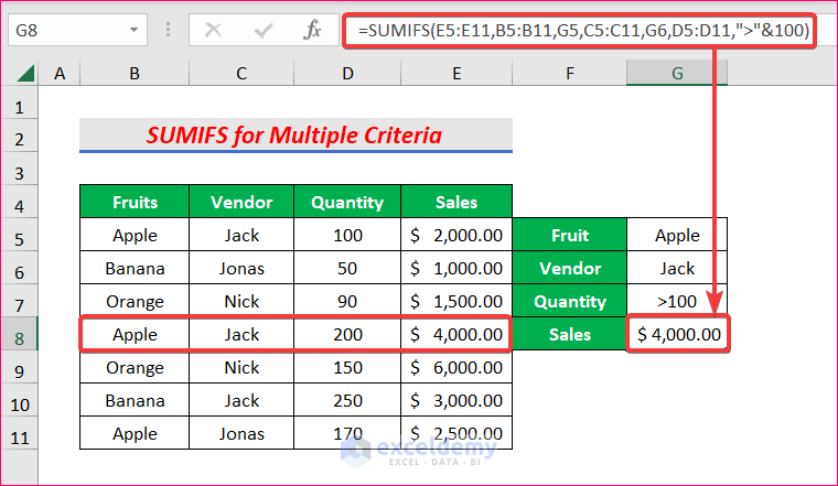
Result:
You will get the total sales for Apple as Fruit, Vendor as Jack, and Quantity greater than 100.
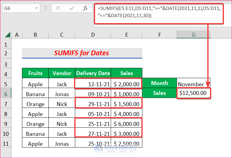
Method 2 – Using the SUMIFS Function for a Date Range
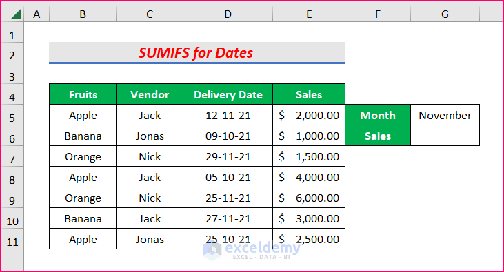
Step 1:
- The output cell is G6.
- Enter the following formula in G6.
=SUMIFS(E5:E11,D5:D11,">="&DATE(2021,11,1),D5:D11,"<="&DATE(2021,11,30))E5:E11 is the range of Sales, D5:D11 is the criteria range which includes the Dates.
">="&DATE(2021,11,1) is the first criteria: DATE will return the first date of a month.
"<="&DATE(2021,11,30) is used as the second criteria: DATE will return the last date of a month.
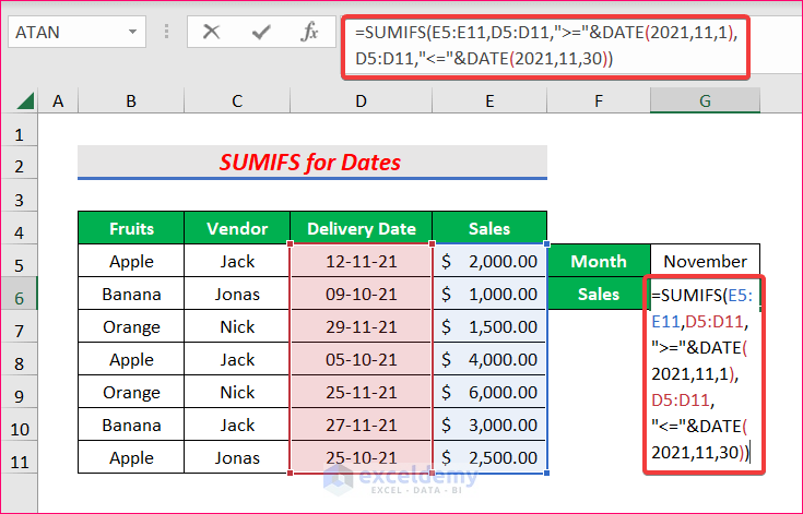
- Press ENTER.
Result:
You will get the sum of sales for November.
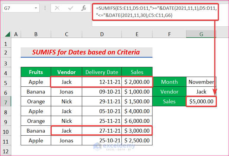
Method 3 – Using the SUMIFS Function for a Date Range based on Criteria
You want to sum Jack’s Sales in November.
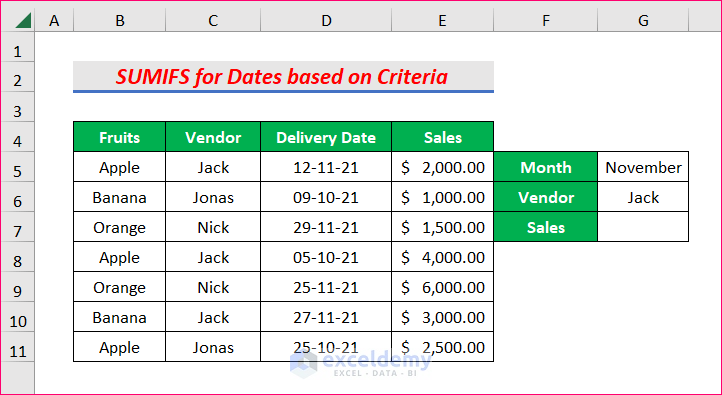
Step 1:
- Enter the following formula in G7.
=SUMIFS(E5:E11,D5:D11,">="&DATE(2021,11,1),D5:D11,"<="&DATE(2021,11,30),C5:C11,G6)E5:E11 is the range of Sales, D5:D11 is the criteria range which includes the Dates.
“>=”&DATE(2021,11,1) is the first criteria: DATE will return the first date of a month.
“<=”&DATE(2021,11,30) is used as the second criteria: DATE will return the last date of a month.
C5:C11 is the third criteria range and G6 is the criteria for this range.

- Press ENTER.
Result:
This is the output.
Method 4 – Using a SUM Array Formula for Multiple Criteria
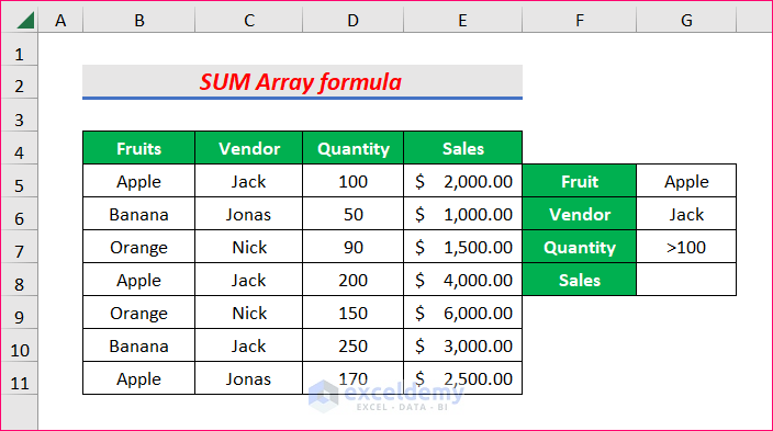
Step 1:
- Enter the following formula in G8.
=SUM((B5:B11="Apple")*(C5:C11="Jack")*(D5:D11>100)*E5:E11)E5:E11 is the sum range
B5:B11=”Apple”, C5:C11=”Jack”, and D5:D11>100 are the three criteria based on which the sales will be added.
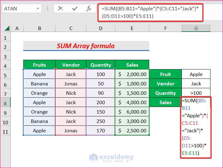
- Press ENTER.
Result:
You will see the total sales for Apple as Fruit, Vendor as Jack, and Quantity greater than 100.
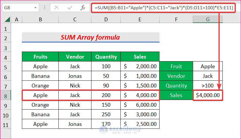
Note:
If you are using a version, other than Microsoft Excel 365, you must press CTRL+SHIFT+ENTER instead of ENTER.
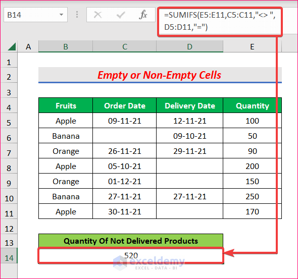
Method 5 – Using the SUMIFS Function for Empty or Non-Empty Cells
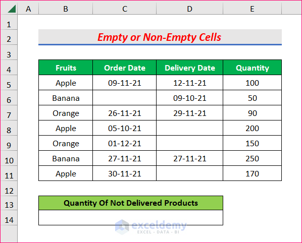
Step1:
- Enter the following formula in the output cell: B14.
=SUMIFS(E5:E11,C5:C11,"<> ",D5:D11,"=")E5:E11 is the sum range
C5:C11 is the range of Order Date and “<> “ is the criteria for this range which means not equal to Blank.
The range of Delivery Date is D5:D11 and “=” is the criteria for this range which means equal to Blank. ( You can use ” ” instead of “=” also)
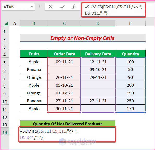
- Press ENTER.
Result:
You will get the Quantity of Not Delivered Products.
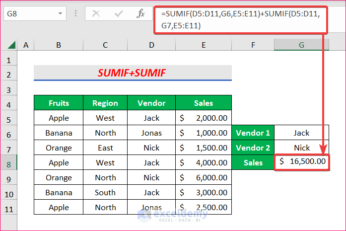
Method 6 – Using the SUMIF + SUMIF function for Multiple OR Criteria
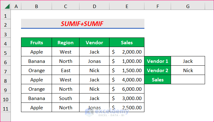
Step 1:
- Enter the following formula in the output cell: G8.
=SUMIF(D5:D11,G6,E5:E11)+SUMIF(D5:D11,G7,E5:E11)This formula will add the Sales values for Vendors Jack and Nick and if one criterion is met, the values will be added.
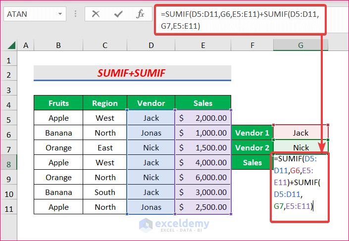
- Press ENTER.
Result:
You will see the Sum of Sales for Jack and Nick.
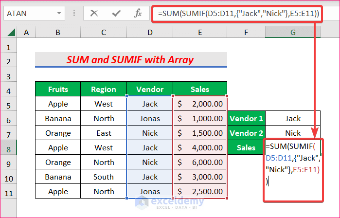
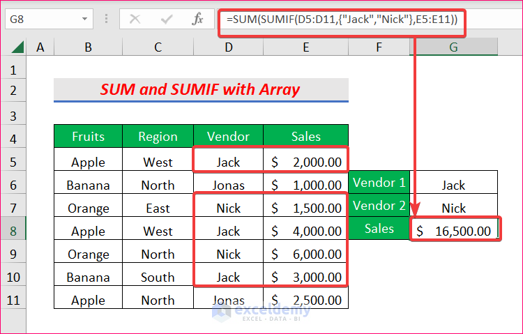
Method 7 – Using the SUM and SUMIF Functions with an Array Formula
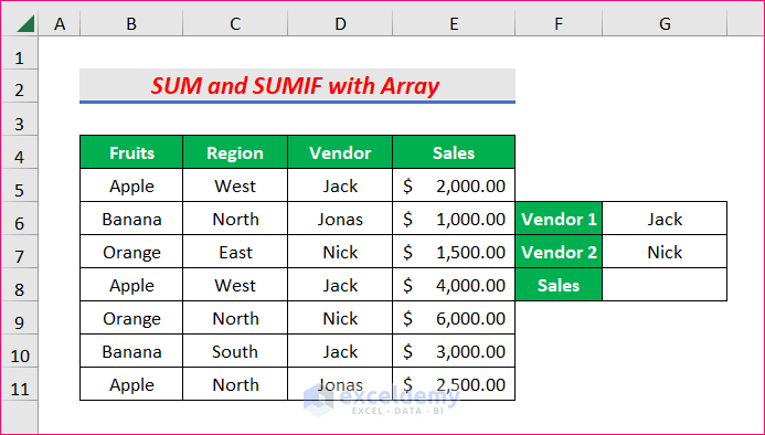
Step 1:
- The output cell is G8.
- Enter the following formula in G8.
=SUM(SUMIF(D5:D11,{"Jack","Nick"},E5:E11))D5:D11 is the criteria range, {“Jack”, “Nick”} is the array of criteria and E5:E11 is the sum range.
Then SUM will add the Sales values for Vendors Jack and Nick and if one criterion is met, the values will be added.
- Press ENTER.
Result:
You will see the Sum of Sales for Jack and Nick.
Note:
If you are using a version, other than Microsoft Excel 365, you must press CTRL+SHIFT+ENTER instead of ENTER.
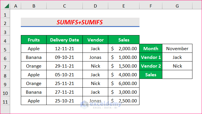
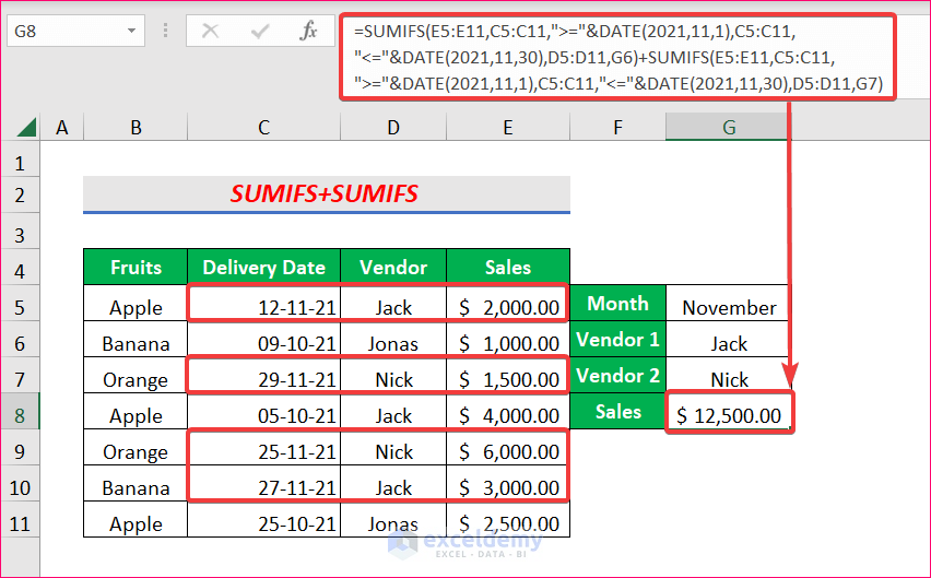
Method 8 – Using the SUMIFS + SUMIFS formula with Multiple Criteria
Step 1:
- The output cell is G8
- Enter the following formula in G8.
=SUMIFS(E5:E11,C5:C11,">="&DATE(2021,11,1),C5:C11,"<="&DATE(2021,11,30),D5:D11,G6)+SUMIFS(E5:E11,C5:C11,">="&DATE(2021,11,1),C5:C11,"<="&DATE(2021,11,30),D5:D11,G7)The two SUMIFS functions will add Sales value for Jack and Nick in November.
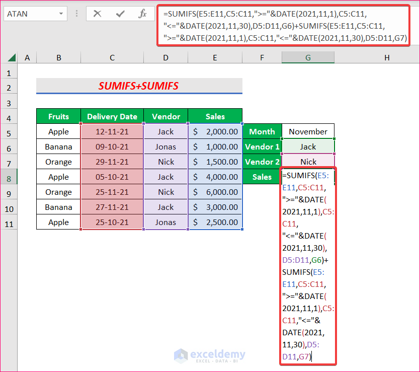
- Press ENTER.
Result:
You will see the Sum of Sales for Jack and Nick in November.
Method 9 – Using the SUMPRODUCT and the SUMIF Function for Multiple Criteria
Step 1:
- Enter the following formula in the output cell: G8.
=SUMPRODUCT(SUMIF(D5:D11,G6:G7,E5:E11))D5:D11 is the criteria range, G6:G7 is multiple criteria in a range and E5:E11 is the sum range.
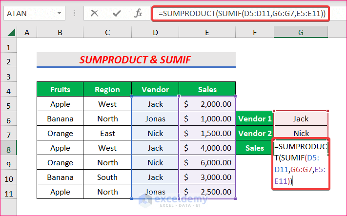
- Press ENTER.
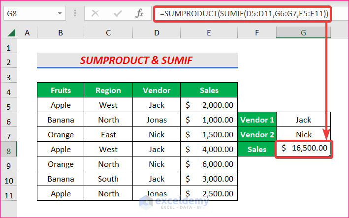
Result:
You will see the Sum of Sales for Jack and Nick.
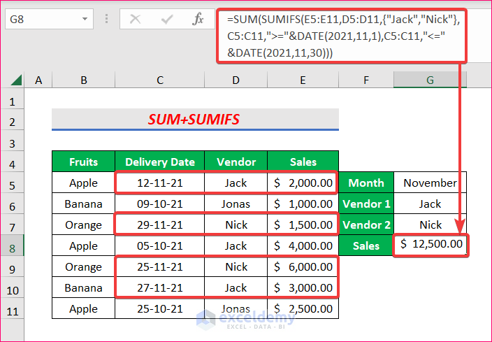
Method 10 – Using the SUM and the SUMIFS Function with an Array
Step 1:
- Enter the following formula in the output cell: G8.
=SUM(SUMIFS(E5:E11,D5:D11,{"Jack","Nick"},C5:C11,">="&DATE(2021,11,1),C5:C11,"<="&DATE(2021,11,30)))D5:D11 is the first criteria range, {“Jack”, “Nick”} is the array of criteria and E5:E11 is the sum range.
C5:C11 is the second and third criteria range
">="&DATE(2021,11,1) is the second criteria: DATE will return the first date of a month.
"<="&DATE(2021,11,30) is used as the third criteria : DATE will return the last date of a month.
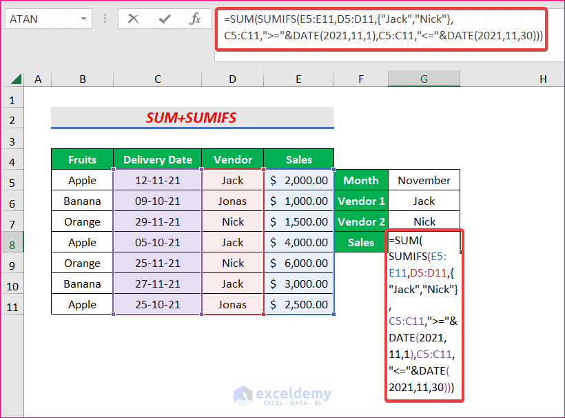
- Press ENTER.
Result:
You will get the Sum of Sales for Jack and Nick in November.
Note:
If you are using a version, other than Microsoft Excel 365, you must press CTRL+SHIFT+ENTER instead of ENTER.
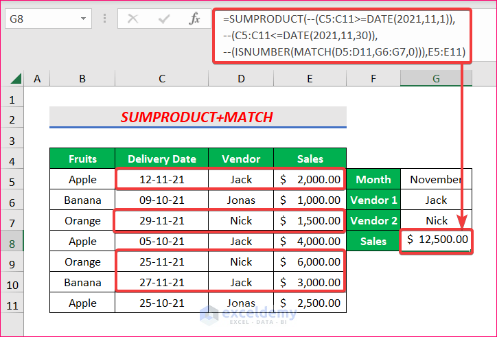
Method 11 – Using the SUMPRODUCT and the MATCH Functions for Multiple Criteria
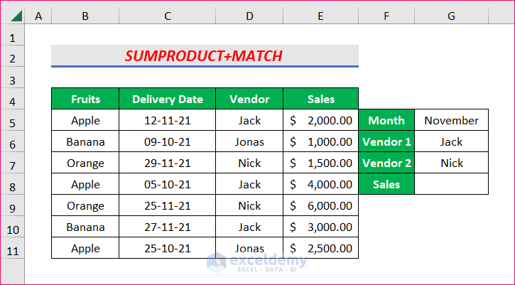
Step 1:
- Enter the following formula in the output cell: G8.
Within the SUMPRODUCT function, there are three criteria, if they are fulfilled, it will return TRUE. Otherwise, FALSE. To convert the criteria into 1 or 0, a double negation(–) was used.
MATCH(D5:D11, G6:G7,0) matches Jack and Nick in the Vendor’s range.
ISNUMBER checks whether there is a number, and returns TRUE or FALSE.
After matching all the criteria, the SUMPRODUCT will add the values in E5:E11.
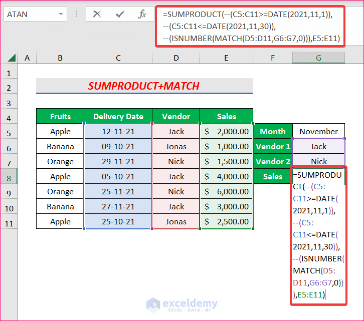
- Press ENTER.
Result:
You will see the Sum of Sales for Jack and Nick in November.
Download Practice Workbook
Get FREE Advanced Excel Exercises with Solutions!
