How to Create Excel Drop Down List from Table (5 Methods)

Method 1 – Creating a Drop-Down List from a Table with Validation

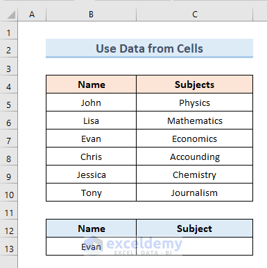
To create a drop-down list from a table, we can use the validation option. This is one of the easiest methods for creating a drop-down. Let’s walk through the steps using the example of a dataset containing students and their subjects:

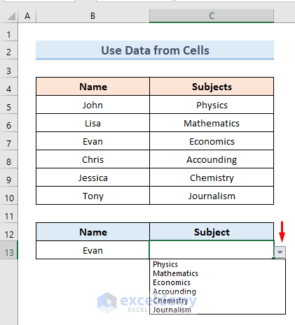
1. Using Cell Data to Create a Drop-Down:

• Begin by selecting cell C13.

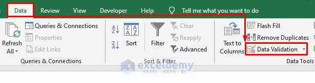
• Go to the Data tab.
• Choose the Data Validation option from the Data Tools section. A new window will open.

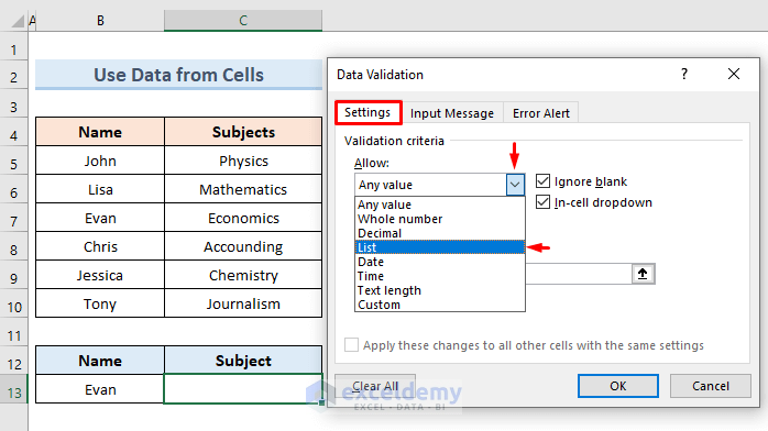
• In the Data Validation window, go to the Settings option.
• Under the Allow section, select the List option from the dropdown.

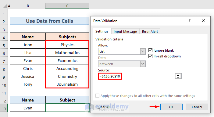
• In the Source field, select the range of cells (C5:C10) that contain the subject values.
• Click OK.

You’ll now see a drop-down icon in cell C13. Clicking on the icon will display the subject values from our dataset.

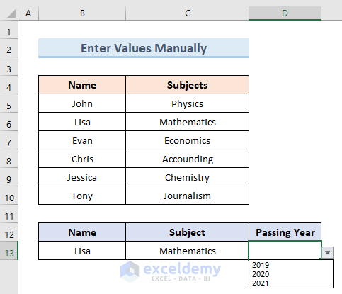
2. Manually Entering Data for the Drop-Down:

In this example, we will manually enter the values for the drop-down, whereas in the previous example, we extracted the values from our dataset. Let’s create a drop-down for the passing year of students in cell D13 using the following steps:

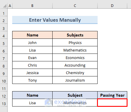
• Begin by selecting cell D13.
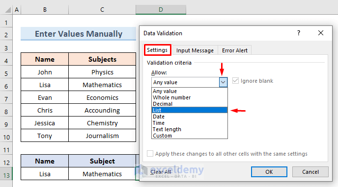
• Open the Data Validation window.
• Go to the Settings option.
• From the Allow drop-down, select the List option.

• In the Source field, manually input the years 2019, 2020, and 2021.
• Press OK.

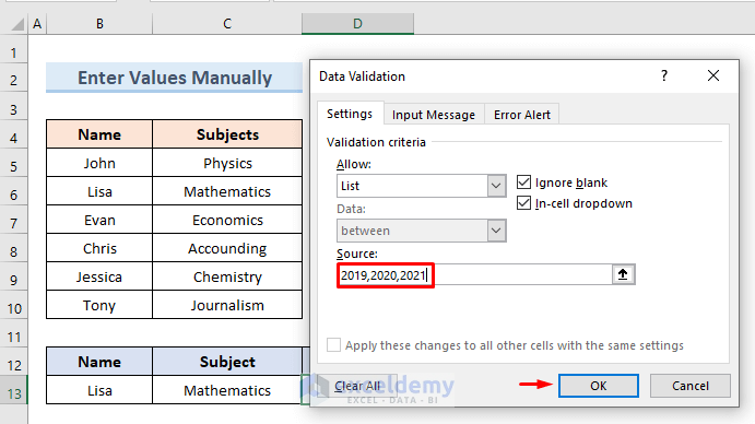
• You’ll now see a drop-down with three values representing the years in cell D13.

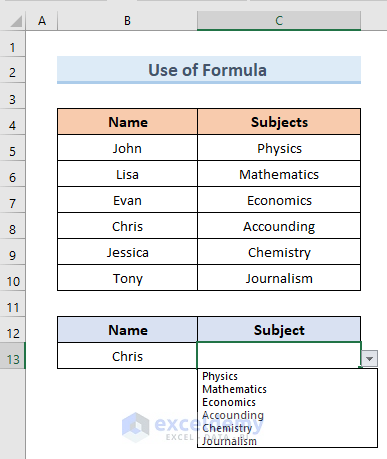
3. Using an Excel Formula

We can also create a drop-down in Microsoft Excel using a formula. In this example, we’ll perform the same task with the same dataset as in the first method. However, this time we’ll use an Excel formula. Let’s walk through the steps:

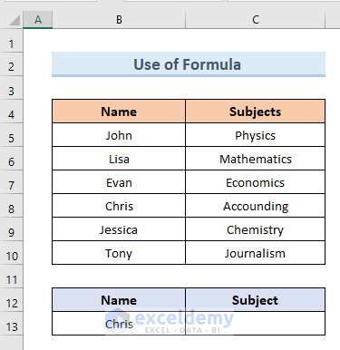
• Begin by selecting cell C13.
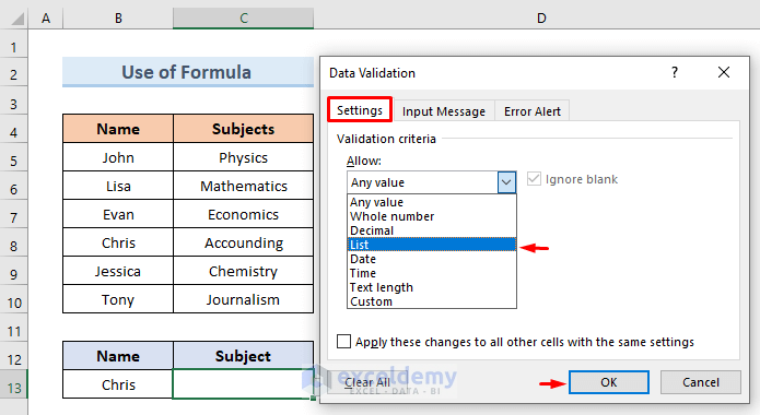
• Open the Data Validation window.
• Choose the Settings option.
• Select the List option from the Allow drop-down.

• In the Source field, insert the following formula containing the OFFSET function
  
  =OFFSET($C$5,0,0,6)
  
• Press OK.

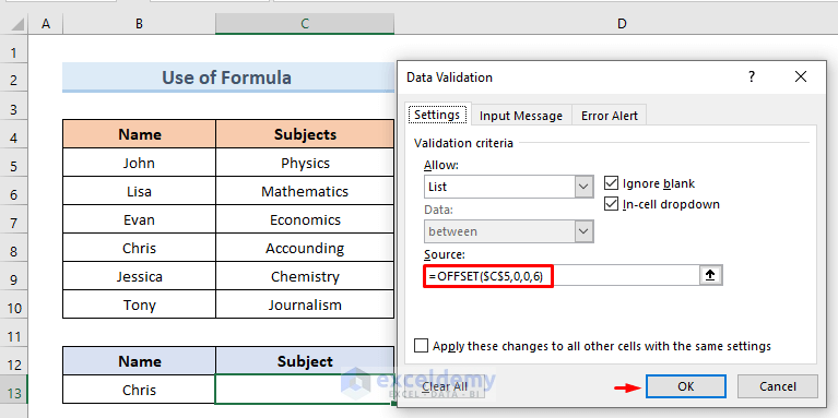
• You’ll now see a drop-down icon in cell C13. Clicking on the icon will display the dropdown list of subjects.

Read More: How to Make a Drop Down List in Excel

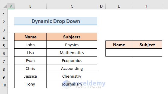
Method 2 – Creating a Dynamic Drop-Down List from an Excel Table

Sometimes, after setting up a drop-down list, we may need to add new items or values to that list. To achieve this, we’ll make the drop-down list dynamic. Follow these steps:

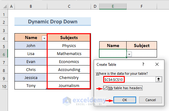
1. Insert a Table:
   • Go to the Insert tab.
   • Select the Table option.
     
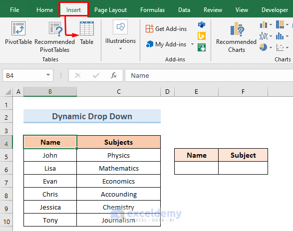
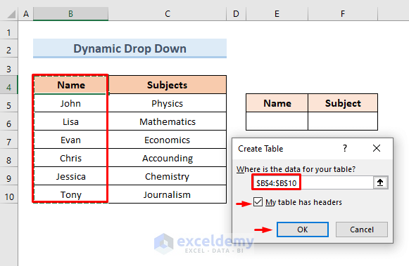
   • A new window will open.
   • Choose the cell range (B4:B10) as your table data.
   • Make sure to check the option “My table has headers.”
   • Press OK.
     
2. Create a Dynamic Drop-Down for the “Name” Column:
   • Select cell E6.
   • Open the Data Validation
   • Choose the Settings
   • Select List from the Allow drop-down.
   • In the new Source bar, insert the following formula:
     
     =INDIRECT("Table1[Name]")
     
   • Press OK.
     
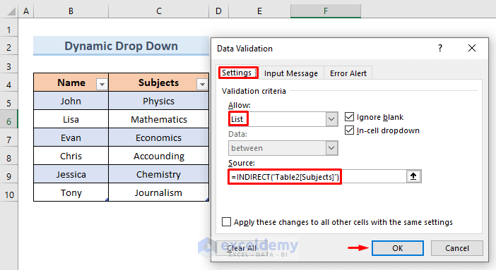
3. Create a Dynamic Drop-Down for the “Subjects” Column:
   • Again, create a table for the Subjects
     
   • Select cell F6.
   • Open the Data Validation
   • Choose the Settings
   • Select List from the Allow drop-down.
   • In the new Source bar, insert the following formula:
     
     =INDIRECT("Table2[Subjects]")
     
   • Press OK.
     
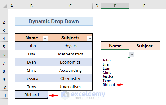
4.  Test the Dynamic Drop-Downs:
   • Add a new name (e.g., “Richard”) in the Name The drop-down list should also display the new value.
     
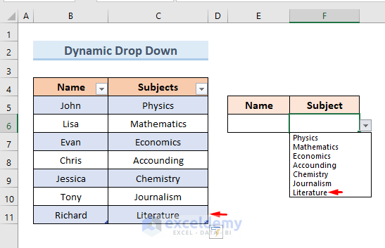
   • Finally, insert a new value (e.g., “Literature”) in the Subjects You should see the new value in the dropdown as well.

Read More: How to Link a Cell Value with a Drop Down List in Excel

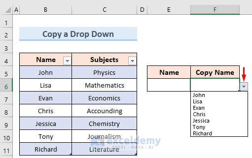
Method 3 – Copying a Drop-Down List in Excel

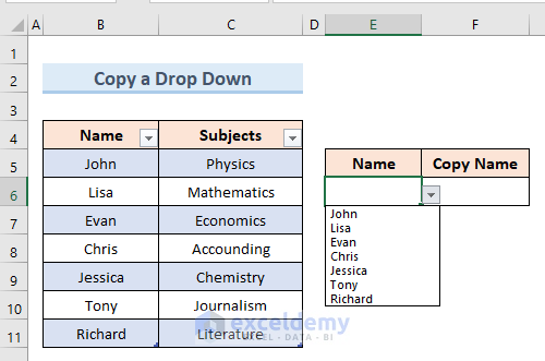
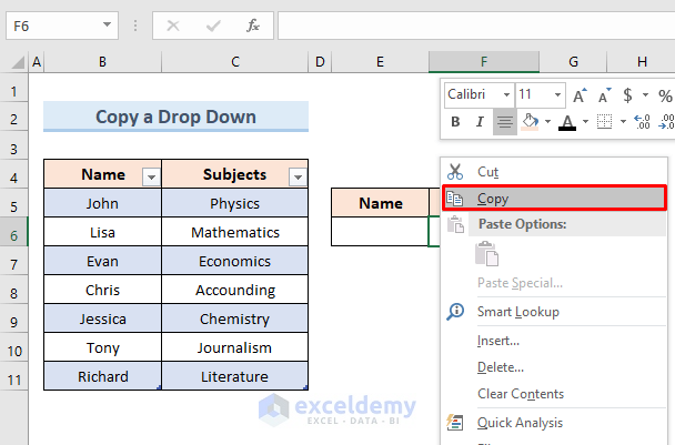
• First, select the cell containing the drop-down list that you want to copy.
• Right-click on the selected cell and choose the Copy

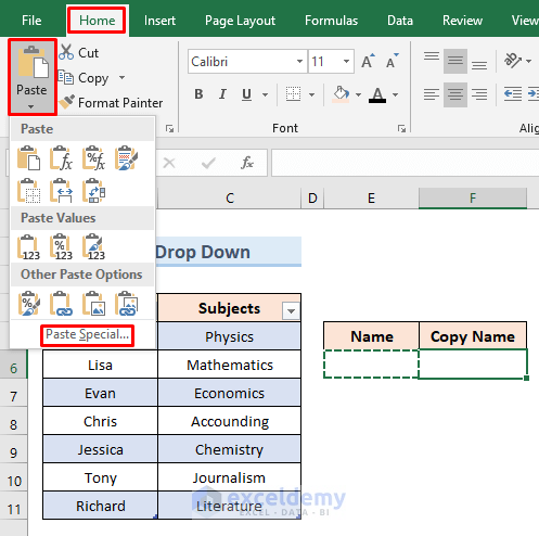
• Next, navigate to the cell where you want to paste the drop-down list (e.g., cell F6).
• Go to the Home tab in the Excel ribbon.
• Click on the Paste option, and from the drop-down menu, select Paste Special.

• A new window will appear. Check the Validation option in the box.
• Press OK”

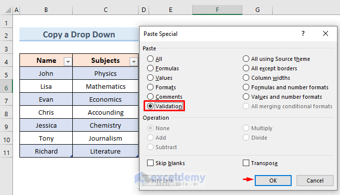
• You’ll now see that the drop-down list in cell F6 is a copy of the one from cell E6.

Read More: How to Copy Filter Drop-Down List in Excel

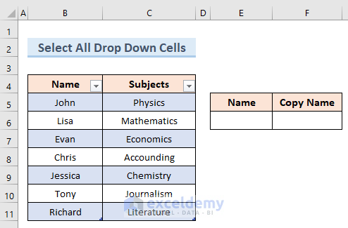
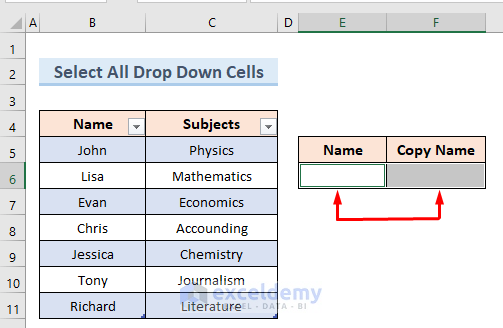
Method 4 – Select All Drop-Down List Cells from a Table

Sometimes, our dataset contains multiple drop-down lists. In this example, we’ll explore how to find and select all the drop-down lists within a dataset. We’ll use the dataset from our previous example to illustrate this method. Follow these simple steps:

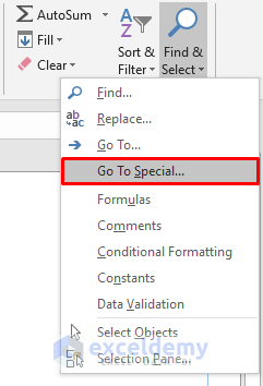
1. Navigate to the “Find & Select” Option:
   • Click on the Find & Select button located in the editing section of the ribbon.
2. Choose “Go To Special”:
   • From the drop-down menu, select the Go To Special
     
   • A new window will appear.
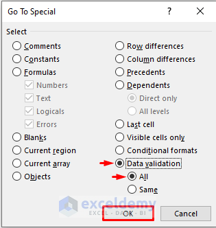
3. Select the “All” Option Under Data Validation:
   • In the “Go To Special” window, check the box labeled All under the Data validation
4. Click “OK”:
   • Confirm your selection by clicking the OK
     

By following these steps, you’ll be able to identify and select all the cells containing drop-down lists in your dataset. In your specific example, this method would result in selecting cells E6 and F6 where the drop-down lists are located.

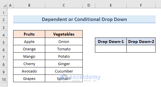
Method 5 – Creating Dependent or Conditional Drop-Down Lists

Suppose we need to create two interrelated dropdown lists. In this example, we’ll explore how to make a drop-down list available depending on another drop-down list. Follow these steps to achieve this:

1. Select Cell E6:
   • Begin by selecting cell E6.
2. Open the Data Validation Window:
   • Open the Data Validation
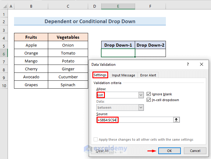
3. Configure the Main Drop-Down List:
   • In the Data Validation dialog box, go to the Settings
   • Under Allow, select “List.”
   • In the Source field, input the following formula:
     
     =$B$4:$C$4
     
   • Click OK.
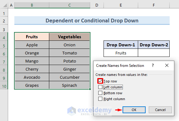
4. Create a Defined Name for the Main List:
   • Go to the Formula
   • Select Create from Selection from the Defined Names
     
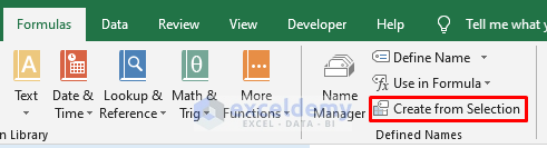
   • In the new window, check only the option for Top row.
   • Press In the new window, check only the option for Top row.
   • Press OK.
     
5. Select Cell F6:
   • Now, select cell F6.
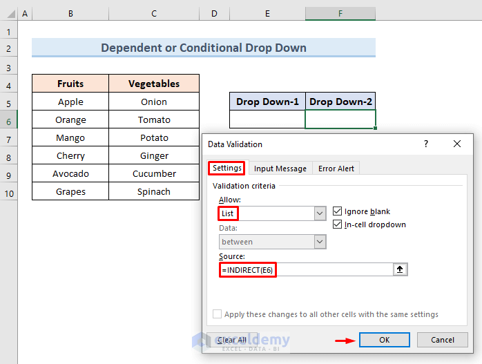
6. Configure the Dependent Drop-Down List:
   • Open the Data Validation window for cell F6.
   • Under Allow, choose the option List.
   • In the Source field, insert the following formula:
     
     =INDIRECT(E6)
     
   • Click OK.
     
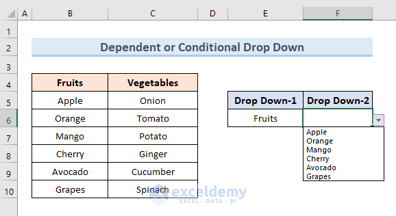
7. Test the Dependent Lists:
   • If you select “Fruits” from Drop Down-1, you’ll see only fruit items in Drop Down-2.
     
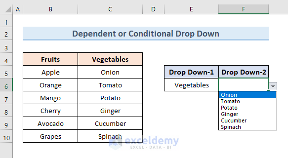
   • Similarly, if you choose “Vegetables” in Drop Down-1, you’ll get the list of vegetables in Drop Down-2.

By following these steps, you’ll create a dependent or conditional drop-down list in Excel.

Read More: Conditional Drop Down List in Excel

Things to Remember

• The drop-down list is lost if you copy a cell (that does not contain a drop-down list) over a cell that contains a drop-down list.
• The worst thing is that Excel will not provide an alert informing the user before overwriting the drop-down menu.

Download Practice Workbook

You can download the practice workbook from here:

Related Articles

• How to Create a Drop Down List from Another Sheet in Excel
• How to Remove Drop Down List in Excel
• How to Auto Update Drop-Down List in Excel
• How to Create Excel Drop Down List with Color
• How to Create Drop Down List with Filter in Excel
• How to Add Item to Drop-Down List in Excel
• How to Create a Drop Down List with Unique Values in Excel
• Excel Drop Down List Not Working

<< Go Back to Create Drop-Down List in Excel | Excel Drop-Down List | Data Validation in Excel | Learn Excel