This tutorial will demonstrate how to create a drop-down list from another sheet in Excel, and also from multiple sheets.
Example 1 – Drop-Down List from A Single Worksheet
Steps:
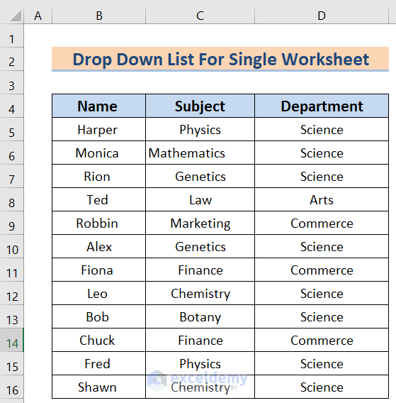
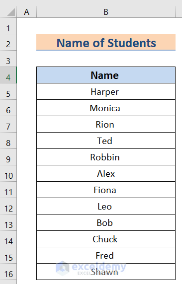
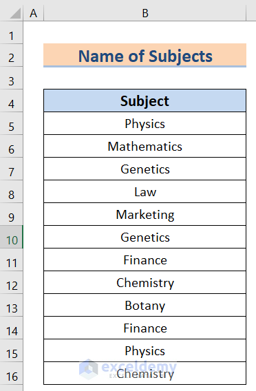
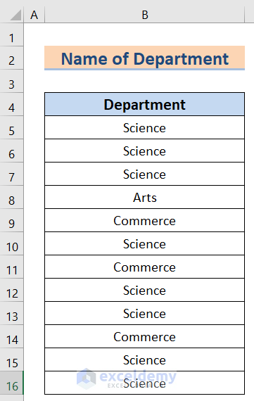
- In a blank worksheet, create the dataset below, containing the Name of some students and their Subject and Department.
- Name the worksheet Source Data.
We’ll make a drop-down list from this data.
- Create a new table in a different worksheet containing columns Name, Subject, and Department.
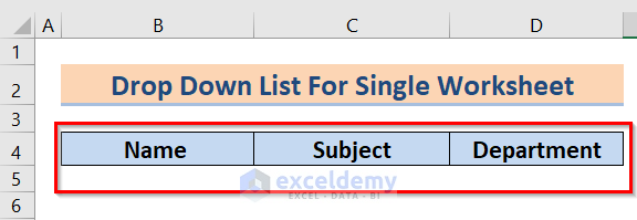
Now we will make a drop-down list for the Names.
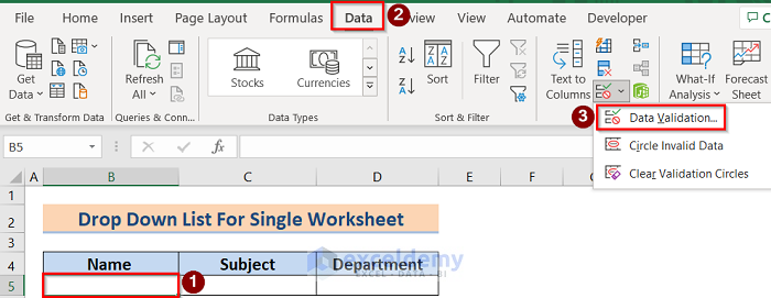
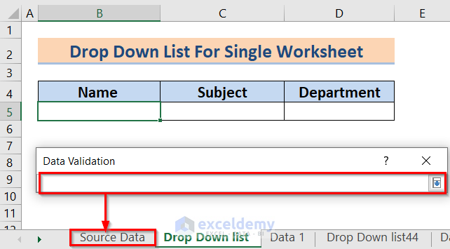
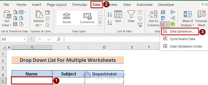
- Select cell B5.
- Go to the Data tab and click on the Data Validation option.
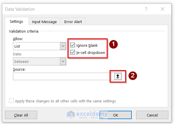
A Data Validation box pops up.
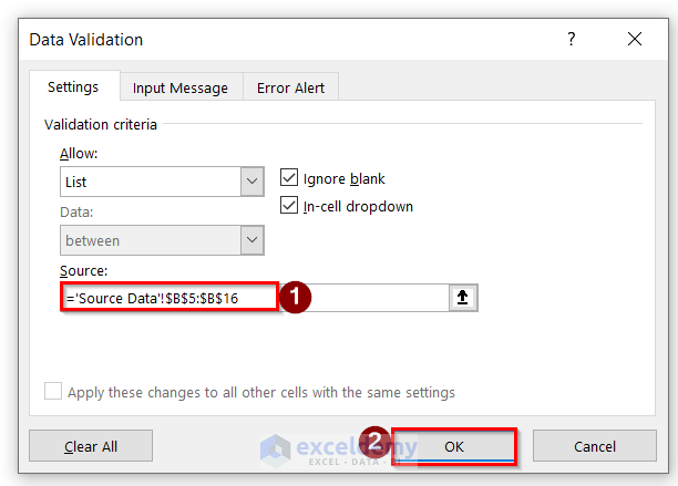
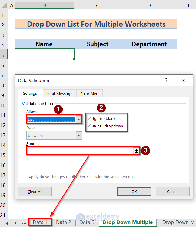
- From the list under Allow:, select the List option.
- Click OK.

- Make sure Ignore Blank and In-cell Dropdown are checked.
- Click on this source icon to select the drop-down list of data.
A new window will appear in which to insert the range containing our drop-down data.
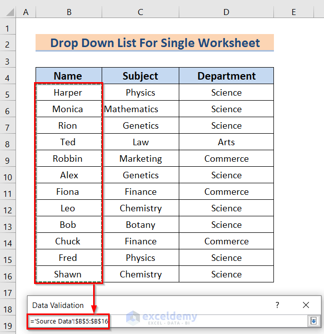
- Click on the Source Data sheet name.
- In the Source Data sheet, select the data in the column Name.
- Click on the data validation icon to confirm the selection.
- Click OK to confirm.
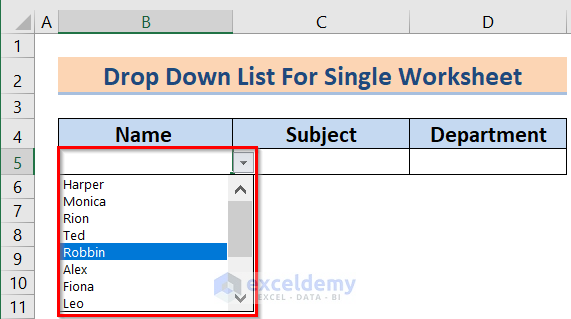
Our drop-down list is ready.
- Click on this icon
 to show the list.
- Repeat the steps for the other two lists.
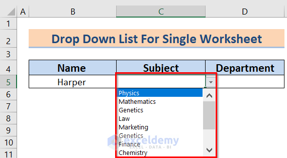
The drop-down list for the Subject column is this:
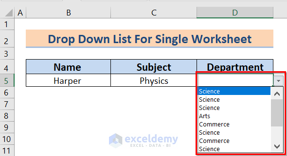
The Department drop-down list is this:
Thus, we have created multiple drop-down lists from data in another sheet.
Read More: How to Make a Drop Down List in Excel
Example 2 – Drop-Down List from Multiple Worksheets
Now let’s create a drop-down list from data in multiple worksheets.
Suppose we have data tables containing the Name, Subject and Department of some students in different sheets. We’ll make drop-down lists in a new worksheet from the data in those sheets.
The Name data is in the sheet named Data 1.
The Subject data is in worksheet Data 2.
And the Department data is in worksheet Data 3.
Steps:
- As in Example 1, make a new table in a new worksheet where the drop-down lists of the data in these sheets will be created.
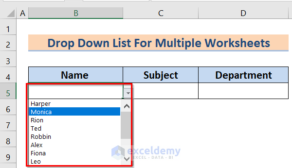
We will first make a drop-down list for the Name column.
- Select the cell range.
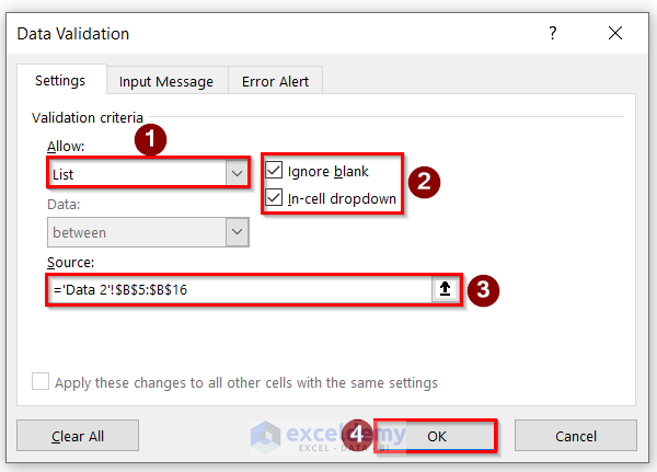
- Go to the Data tab and click on the Data Validation option.
A new window opens.
- Click on this icon to open a chart where different styles of drop-down lists are provided.
- Select List.
- Make sure Ignore Blank and In-Cell Dropdown are checked.
- Click on the source icon to continue.
- Another new window pops out in which to insert the range for our drop-down list.
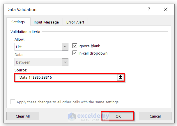
- Go to the Data 1 sheet, select the data and click on the icon to the right in the Data Validation window to continue.

In the new window, the selection is displayed.
- Click OK to proceed.
We have the drop-down list for the Name column.
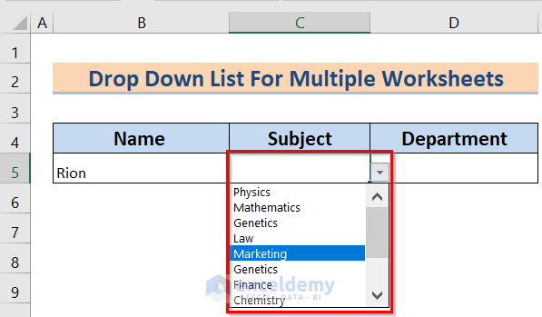
- Do the same for the Subject and Department columns.
The selected range for the Subject column is as follows:
So the drop-down list for the Subject column is as follows:
After repeating the process for the Department column, its drop-down list is as follows:
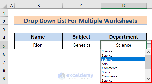
We have successfully created drop-down lists in one table from data in multiple worksheets.
Read More: How to Select from Drop Down and Pull Data from Different Sheet in Excel
Things to Remember
- To avoid errors, remember to check Ignore Blank and In-cell Dropdown.
- If you want the same drop-down list to appear in multiple cells, select those cells and follow the provided procedure.
Download Practice Workbook
Further Reading
- Create Excel Drop Down List from Table
- How to Remove Drop Down List in Excel
- How to Link a Cell Value with a Drop Down List in Excel
- How to Auto Update Drop-Down List in Excel
- How to Create Excel Drop Down List with Color
- How to Create Drop Down List with Filter in Excel
- How to Add Item to Drop-Down List in Excel
- How to Create a Drop Down List with Unique Values in Excel
- How to Copy Filter Drop-Down List in Excel
- Excel Drop Down List Not Working
<< Go Back to Create Drop-Down List in Excel | Excel Drop-Down List | Data Validation in Excel | Learn Excel
Get FREE Advanced Excel Exercises with Solutions!
