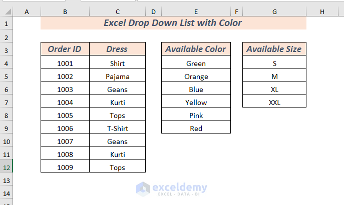
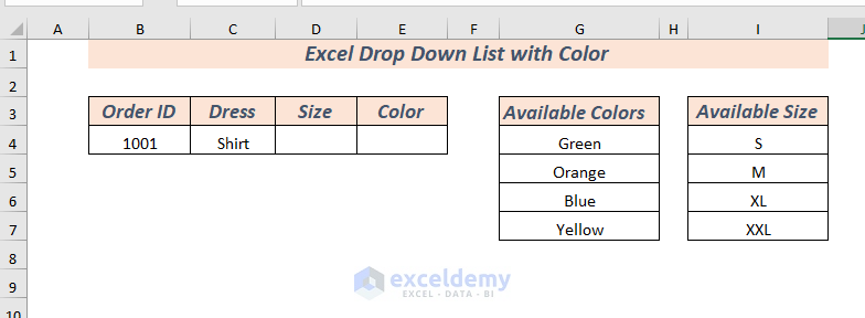
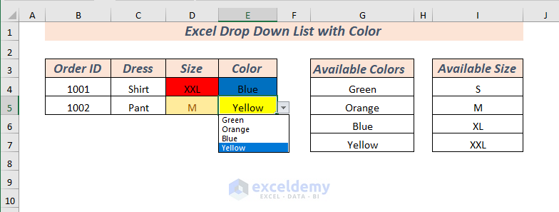
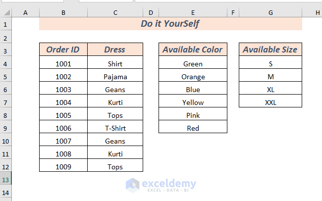
We’ll use a sample dataset of dress stores that represents the order, size, and color information of a particular dress. The dataset contains 4 columns: Order ID, Dress, Available Color, and Available Size.
Method 1 – Creating a Drop-Down List with Color Manually
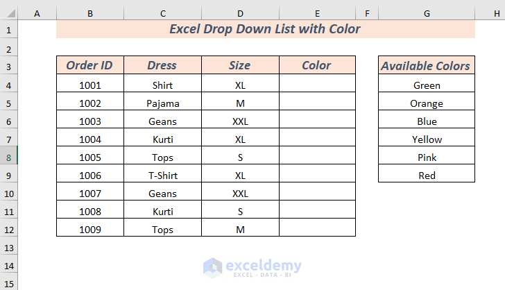
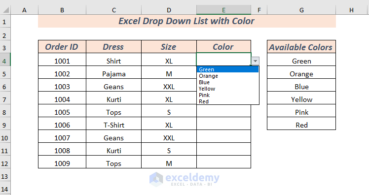
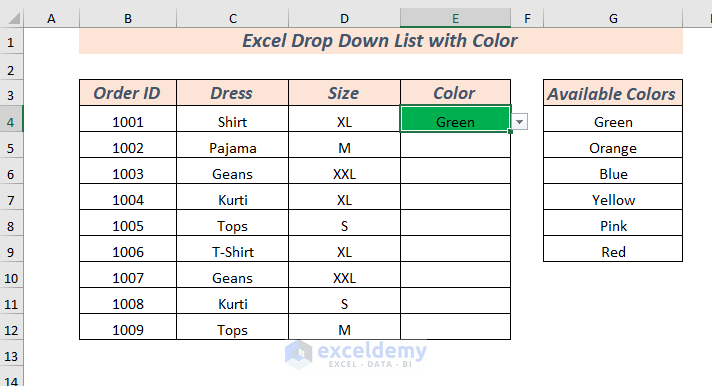
We will create the drop-down list of the Available Colors.
Creating the Drop-Down List
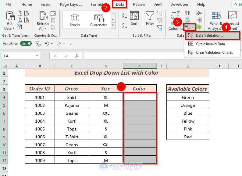
- Select the cell or cell range to apply Data Validation. We selected the cell range E4:E12.
- Open the Data tab.
- From Data Tools, select Data Validation.
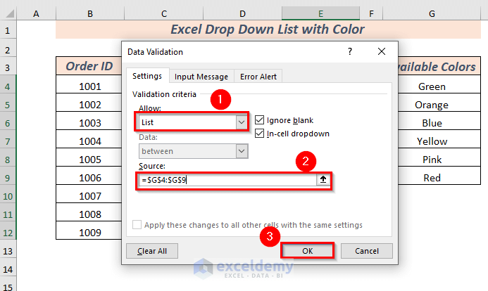
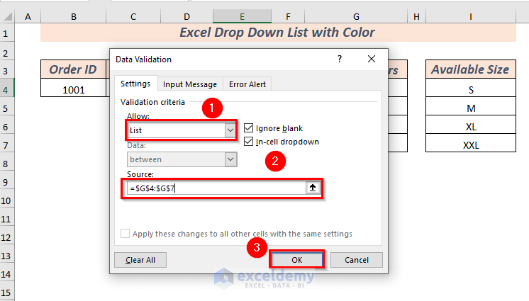
- A dialog box will pop up. For the validation criteria, select the option you want to use in Allow. We selected List.

- Select the source. We selected the source range G4:G9.
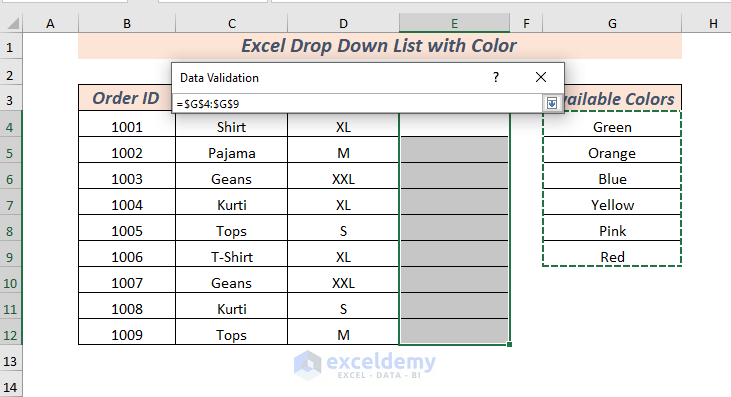
- Click OK.
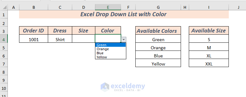
- Data Validation is applied for the selected range.
Read More: How to Make a Drop Down List in Excel
Color the Drop-Down List
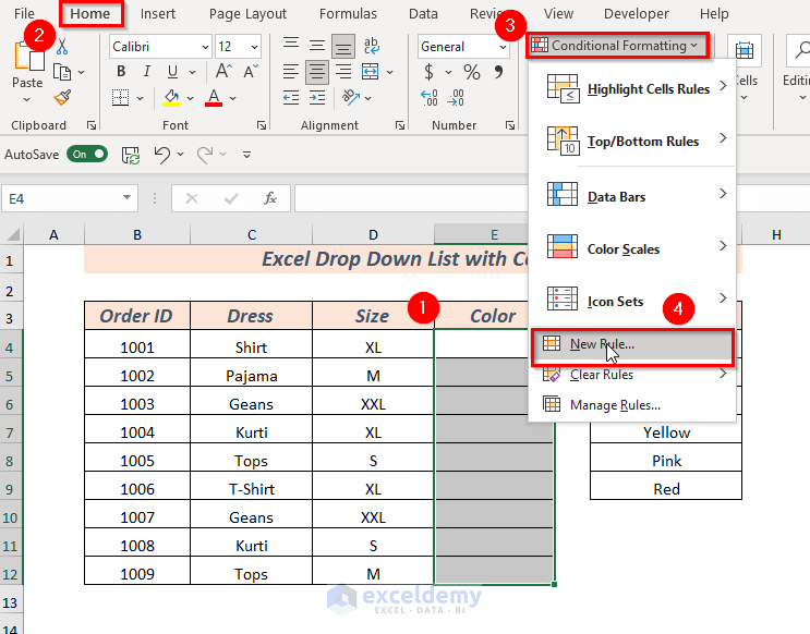
- Select the cell range where Data Validation is applied.
- In the Home tab, select Conditional Formatting and choose New Rule.
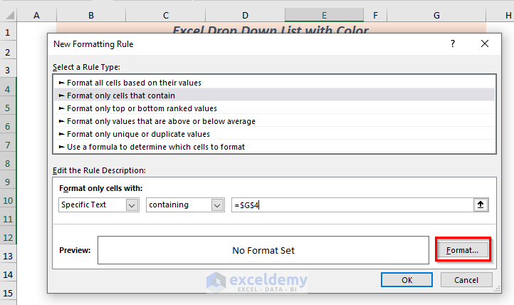
- A dialog box will pop up. Select the rule Format only cells that contain.
- Select the Format only cells with option Specific Text.

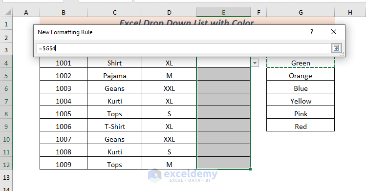
- Select the cell address from the sheet that contains the Specific Text.
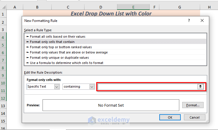
- We selected the G4 cell which contains the color Green.
- Click on Format to set the color of the Specific Text.
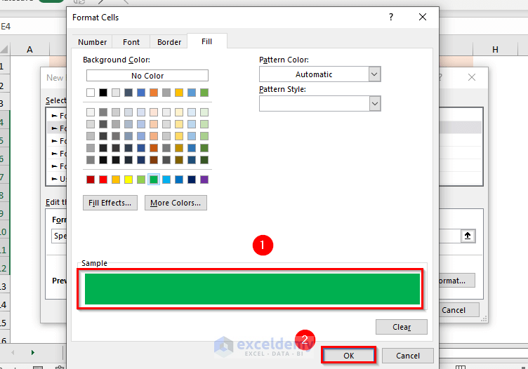
- Another dialog box will pop up. Select the fill color that corresponds to the text value you put as the condition.
- Click OK.
- Click OK again.
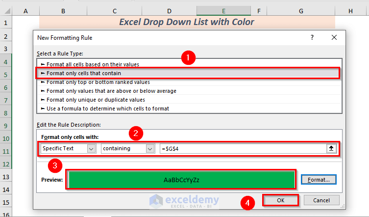
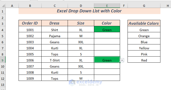
- The specific text Green is colored with green for our example.
- Every time you select the text Green from the drop-down list the cell will be colored with green color.
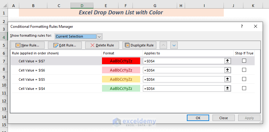
- Repeat the process to add additional fill colors. Apply a New Rule every time, in the same dataset.
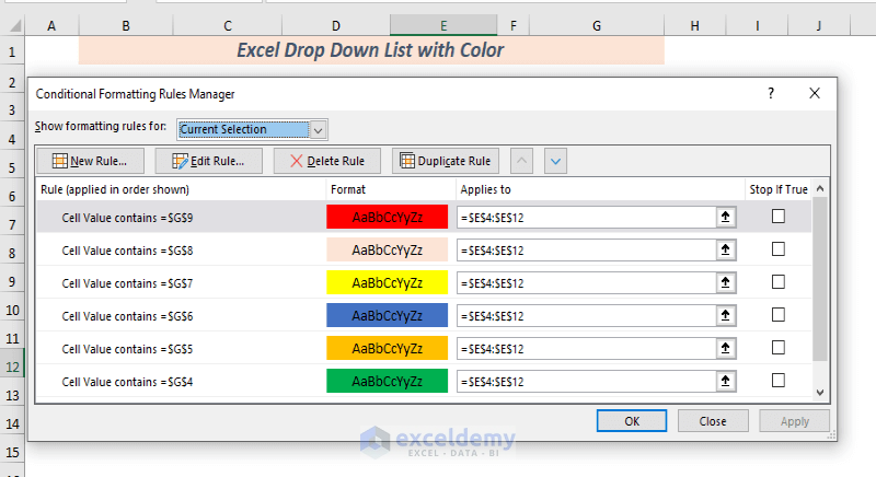
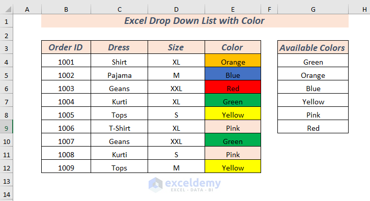
- Each time you select a value from the drop-down list, it will appear with the corresponding color in the cell.
Method 2 – Using the Table Format in Excel to Create a Drop-Down List with Color
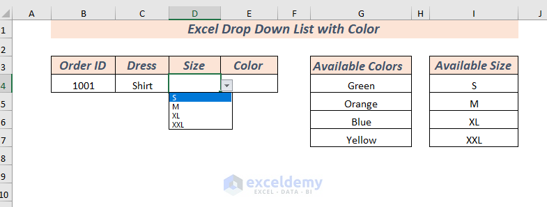
We’ll create two drop-down lists, one for Available Size and another for Available Colors.
Creating the Drop-Down List
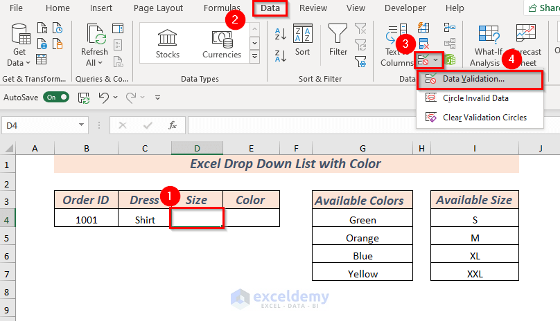
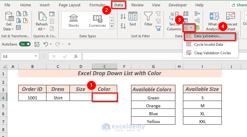
- Select the cell to apply Data Validation. We selected cell D4.
- Open the Data tab and select Data Validation.
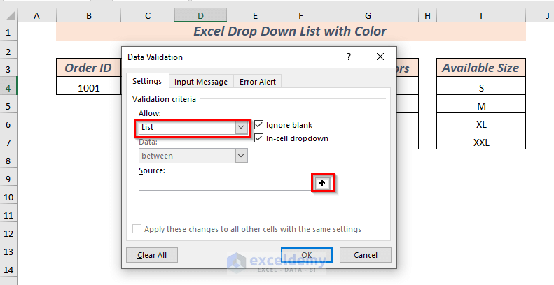
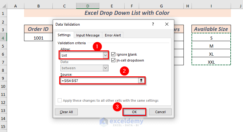
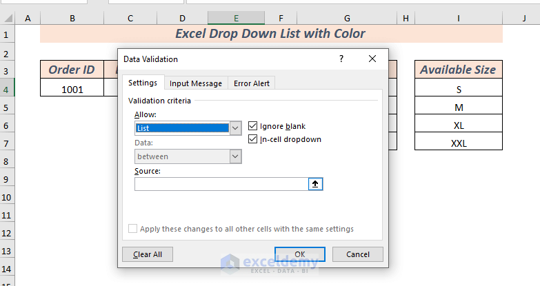
- A dialog box will pop up. For Allow, select List.
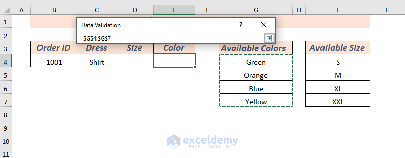
- Select the Source from the sheet.
- We selected the source range I4:I7 as we’re inputting the sizes.
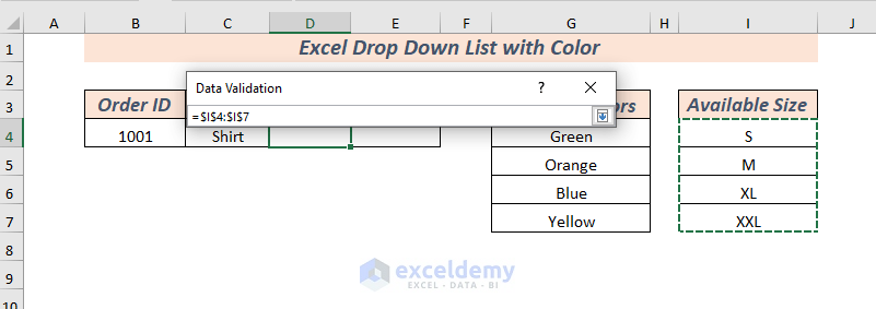
- Click OK.
- You will see Data Validation is applied for the selected cell.
- Repeat the process for cell E4.
- Select a different Source from the sheet, since we need to select colors.
- We selected the source range G4:G7.
- Click OK.
- Data Validation is applied for the selected cell.
Color The Drop-Down List
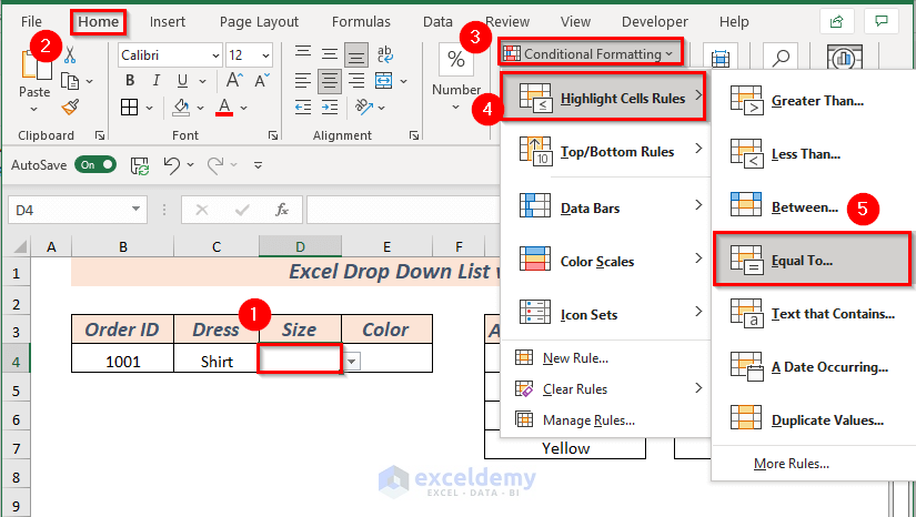
- Select the cell range where Data Validation is applied. We selected cell D4.
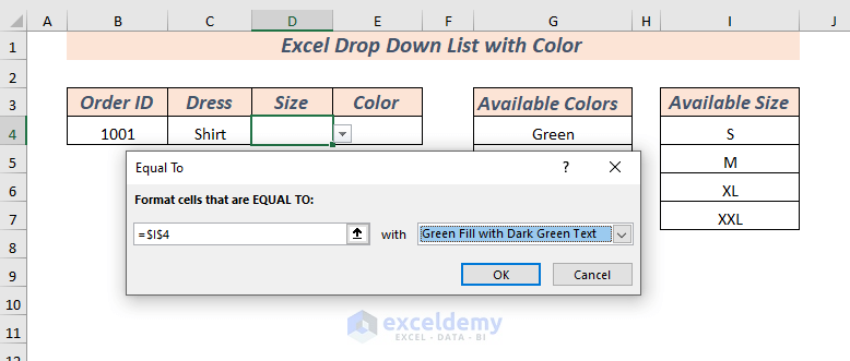
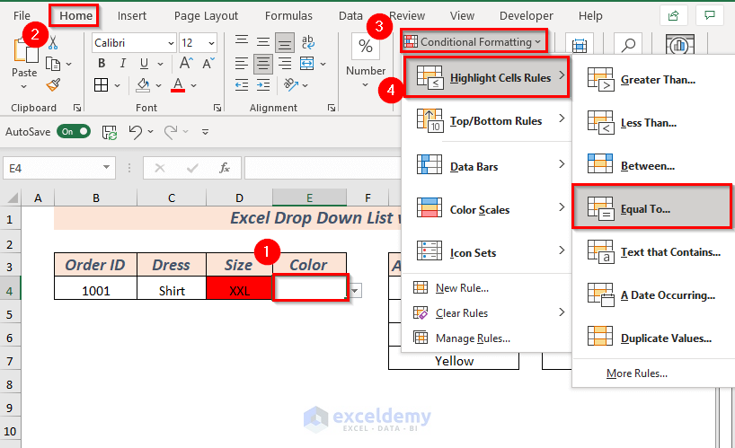
- In the Home tab, go to Conditional Formatting, choose Highlight Cells Rules, and select Equal To.
- A dialog box will pop up. From there select any cell to apply Format cells that are EQUAL TO. We selected cell I4.
- In with, select an option. We selected Green Fill with Dark Green Text.
- Click OK.
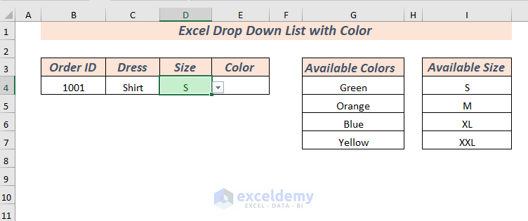
- The size value from the drop-down list is coded with the selected color.
- Repeat this process to color the drop-down list value which is in the I5 cell.
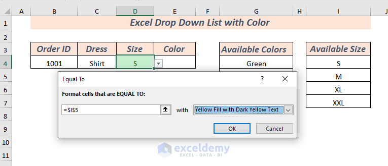
- The I5 value is colored with the followed option.
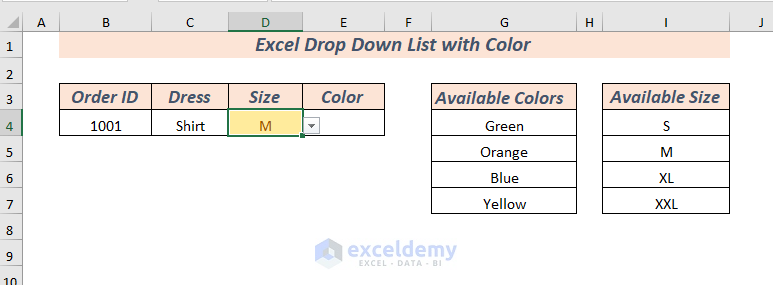
- Repeat the process to color all the drop-down list values of Available Size.
- Select cell E4.
- In the Home tab, go to Conditional Formatting, select Highlight Cells Rules, then choose Equal To.
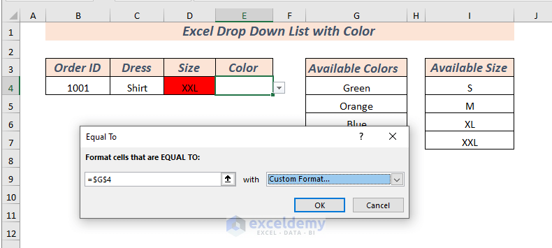
- A dialog box will pop up. Select any cell to apply Format cells that are EQUAL TO. We selected cell G4.
- In with, select an option. We selected Custom Format.
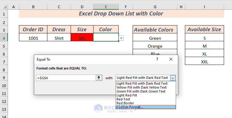
- Another dialog box will pop up. Select the fill color of your choice. We selected the color Green since the condition value points to Green.
- Click OK.
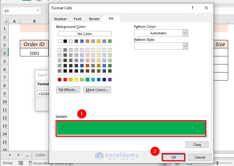
- Click OK.
- The selected color is applied to the drop-down list values.
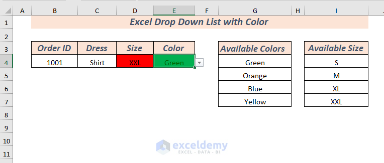
- Repeat to color all the values of Available Colors.
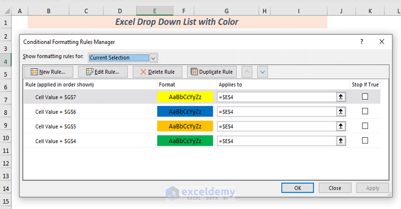
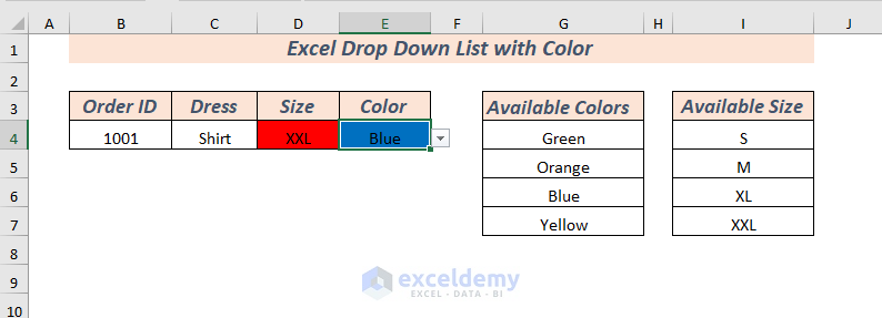
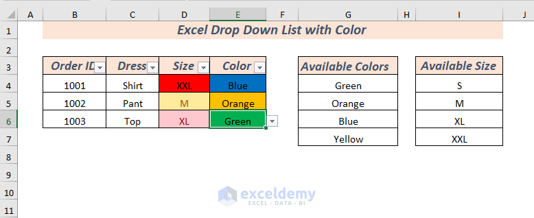
Each of the values will appear with a formatted color.
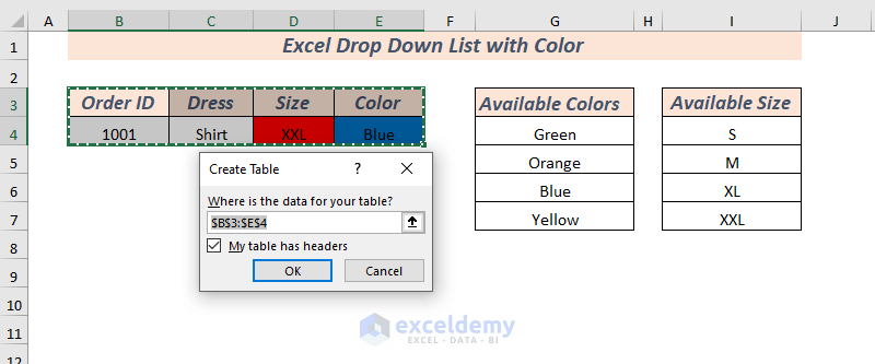
Using the Table Format in a Drop-Down List with Color
- Select the cell range to format the range as Table. We selected the cell range B3:E4.
- Open the Home tab, choose Format as Table, and select any Format (we selected Light)

- A dialog box will appear. Check My table has headers.
- Click OK.
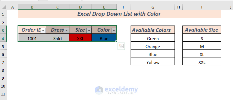
- You will see that the Table format is applied.
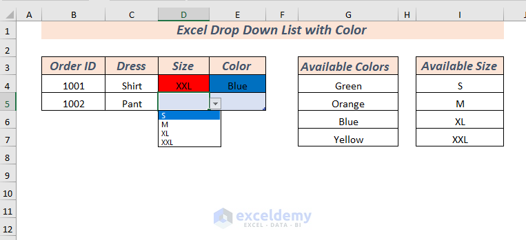
- Insert new data in row 5 and you will see that the drop-down list is available.
- Select any value to check if the values come with colors.
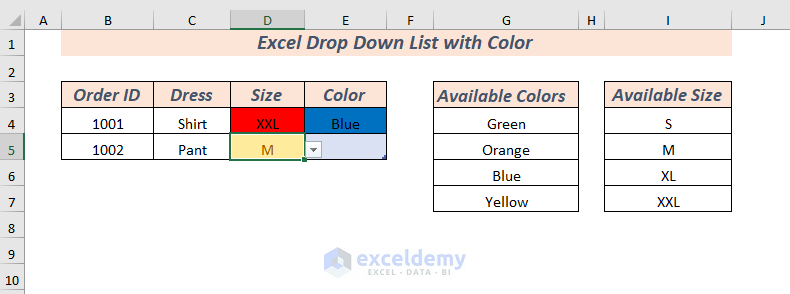
- You will see a drop-down list with color.
- You can add more cells to the table.
If you don’t want the Filter option in the Table Header, you can remove it.
- Select the Table,
- Open the Table Design tab, then from Table Style Options, uncheck Filter Button.
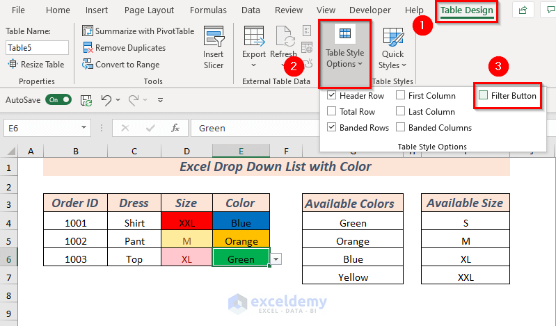
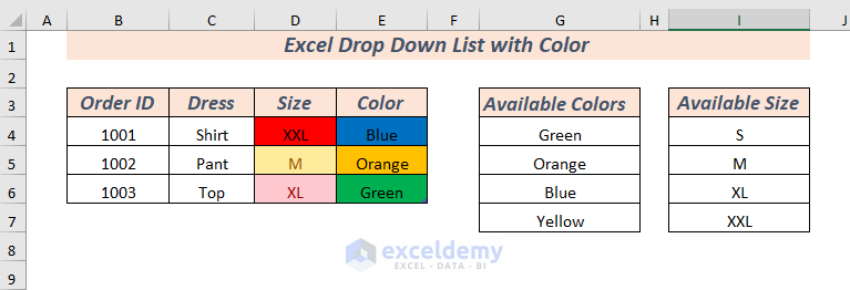
- The table header filter button is removed.
Read More: Create Excel Drop Down List from Table
Practice Section
We’ve provided a practice sheet in the workbook to practice these methods.
Download the Practice Workbook
Related Articles
- How to Create a Drop Down List from Another Sheet in Excel
- How to Remove Drop Down List in Excel
- How to Link a Cell Value with a Drop Down List in Excel
- How to Auto Update Drop-Down List in Excel
- How to Create Drop Down List with Filter in Excel
- How to Add Item to Drop-Down List in Excel
- How to Create a Drop Down List with Unique Values in Excel
- How to Copy Filter Drop-Down List in Excel
- Excel Drop Down List Not Working
<< Go Back to Create Drop-Down List in Excel | Excel Drop-Down List | Data Validation in Excel | Learn Excel
Get FREE Advanced Excel Exercises with Solutions!

Thank you so much, this was quite helpful!!
Hello Vishal Kapadiya,
You are most welcome. Thanks for your feedback and appreciation. Glad to hear that our article is helpful to you.
Keep exploring Excel with ExcelDemy!
Regards
ExcelDemy