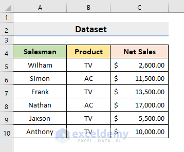
This is the sample dataset:
Method 1 – Create a Drop-Down Filter to Extract Data Based on Selection with Helper Columns in Excel
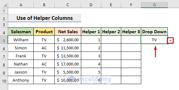
Insert 3 helper columns.
STEPS:
- Select D5 and use the ROW function:
=ROWS($B$5:B5)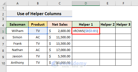
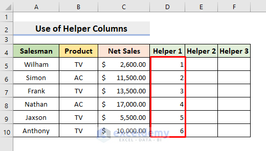
- Press Enter and use the Fill Handle to complete the series.
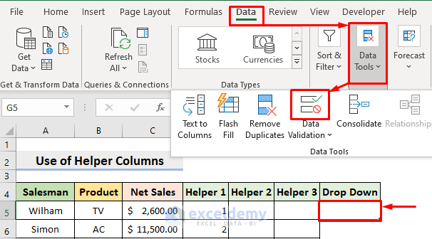
- Select G5 to create the drop-down filter.
- Select Data ➤ Data Tools ➤ Data Validation.
- In the Data Validation dialog box, choose Settings.
- Select List in Allow.
- Enter TV, AC in the Source box.
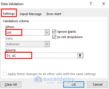
- Click OK.
The filter is created.
- Select E5 and enter the formula:
=IF(B5=$G$5,D5,"")- Press Enter.
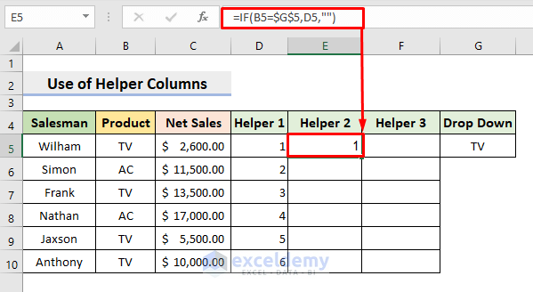
- Drag down the Fill Handle to see the result in the rest of the cells.
- Select F5. Use the formula:
=IFERROR(SMALL($E$5:$E$10,D5),"")- Press Enter.
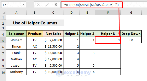
- Drag down the Fill Handle to see the result in the rest of the cells.
- Select I5 and enter the formula:
=IFERROR(INDEX($A$5:$C$10,$F5,COLUMNS($I$5:I5)),"")- Press Enter.
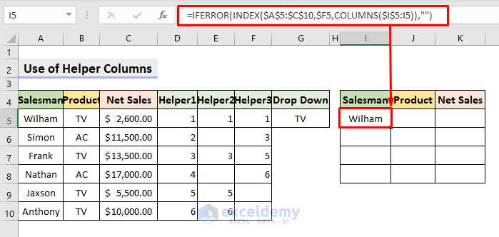
The COLUMNS function returns the number of columns in $I$5:I5. The INDEX function returns the cell reference or cell value at the intersection of the row number in F5 and the column number in I5. The IFERROR function returns blank cells if an error is found.
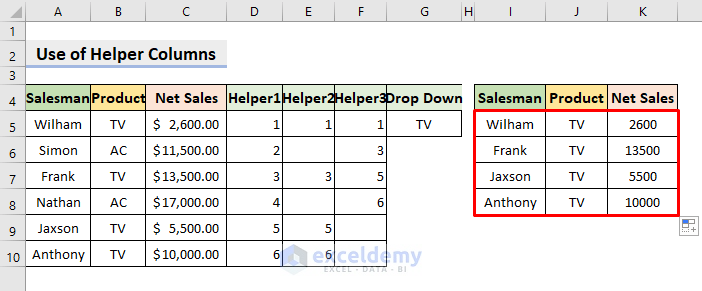
- Drag down the Fill Handle to see the result in the rest of the cells.
This is the output.
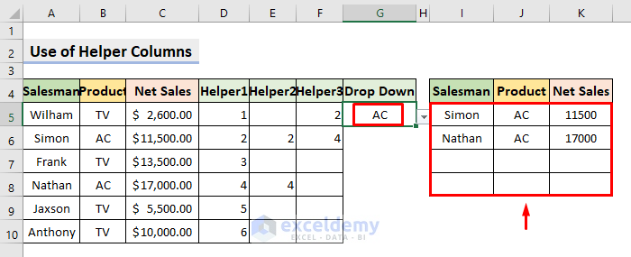
- Choose AC from the drop-down filter, The dataset will automatically update.
Read More: How to Make Multiple Selection from Drop Down List in Excel
Method 2 – Using the FILTER Function to Create a Drop-Down Filter and Extract Data Based on the Selection
STEPS:
- Select A4:C10.
- In the Insert tab, select Table.
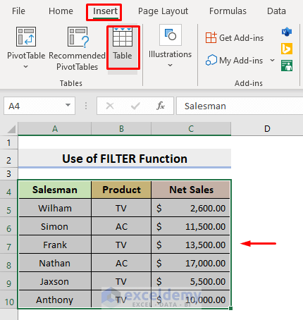
- In the dialog box, click OK.
Table1 is created.
- Open a blank sheet and select B2. Enter the formula:
=UNIQUE(Table1[Product])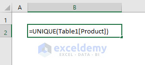
- Click OK.
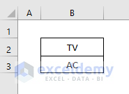
Unique product names are displayed.
- Select E5 in the main sheet.
- Go to Data ➤ Data Tools ➤ Data Validation.
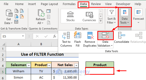
- In the dialog box, choose Settings.
- Select List in Allow.
- In the Source box, enter the formula:
=list!$B$2#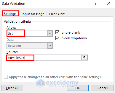
list is the new sheet name. The formula will look for the value in B2 in the list sheet.
- Select G5. Use the formula:
=FILTER(Table1,Table1[Product]=E5)- Press Enter.
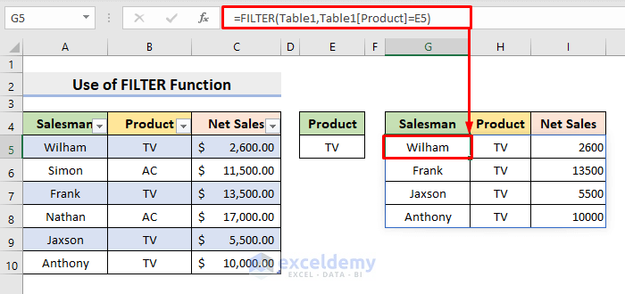
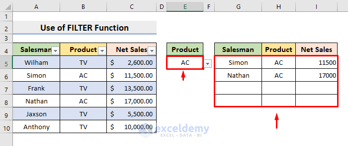
The FILTER function filters Table1 and returns the dataset that matches E5.
- Change the drop-down filter to AC to see the output.
Read More: Create a Searchable Drop Down List in Excel
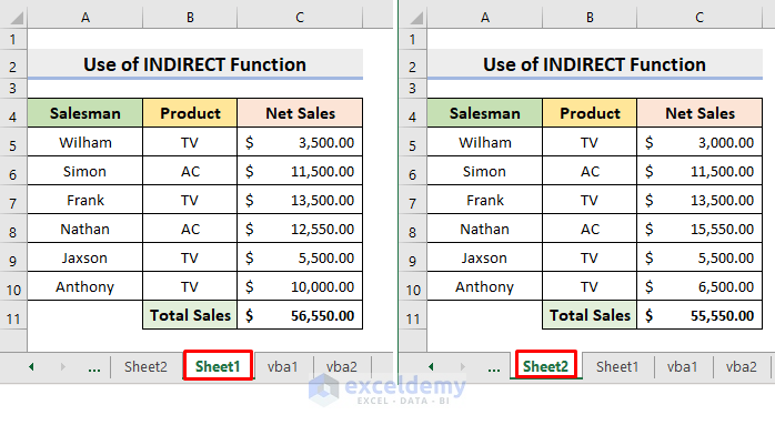
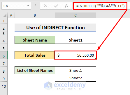
Method 3 – Extract Data Based on a Selection by Creating a Drop Down Filter with the INDIRECT Function
To extract the Total Sales based on a selection:
STEPS:
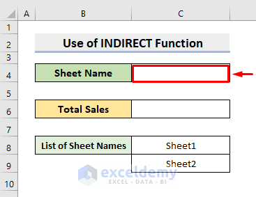
- Select C4 in the sheet you want to place the extracted data.
- Select Data ➤ Data Tools ➤ Data Validation.
- In the dialog box, select List in Allow.
- In the Source box, enter the formula:
=$C$8:$C$9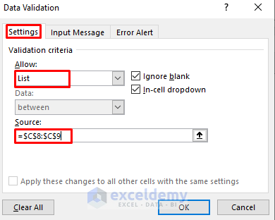
- Click OK.
- Select C6 and use the formula:
=INDIRECT("'"&C4&"'!C11")- Press Enter.
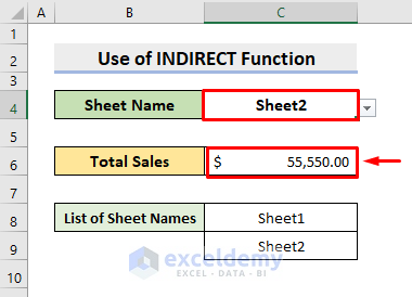
The Total Sales in the selected sheet are displayed in C4.
- Change the sheet using the drop-down filter. You’ll see the change in C6.
Method 4 – Using VBA to Create a Drop Down Filter and Extract Data Based on a Selection in Excel
STEPS:
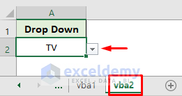
- The dataset is in the vba1 sheet.
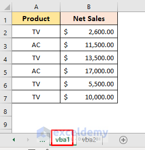
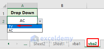
- The drop-down filter is in the vba2 sheet. To filter data in the vba1 sheet according to the drop-down selection in the vba2 sheet.
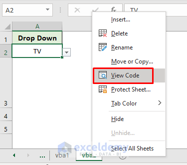
- Right-click the vba2 sheet.
- Select View Code.
- In the Module window, enter the code below:
Private Sub Worksheet_Change(ByVal Target As Range)
    On Error Resume Next
    If Not Intersect(Range("A2"), Target) Is Nothing Then
        Application.EnableEvents = False
        If Range("A2").Value = "" Then
            Worksheets("vba1").ShowAllData
        Else
            Worksheets("vba1").Range("A2").AutoFilter 1, Range("A2").Value
        End If
        Application.EnableEvents = True
    End If
End Sub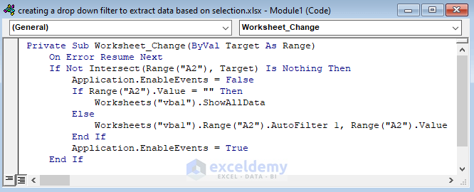
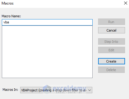
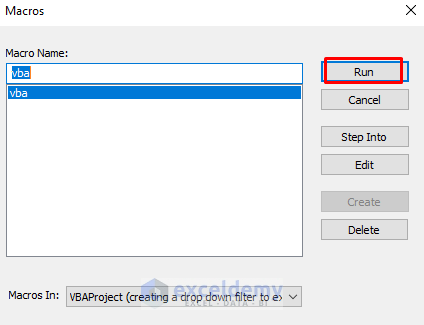
- Press F5.
- In the Macros dialog box, enter VBA in Macro Name:.
- Click Create.
- Press F5 and select Run.
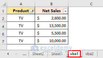
- Close the window. From the Drop-Down Filter, select TV.
You’ll see the filtered data in the vba1 sheet.
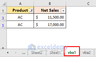
Select AC from the drop-down filter in the vba2 sheet to see the extracted data.
Download Practice Workbook
Download the following workbook.
Related Articles
- How to Create Drop Down List in Multiple Columns in Excel
- How to Add Blank Option to Drop Down List in Excel
- How to Create a Form with Drop Down List in Excel
- How to Remove Used Items from Drop Down List in Excel
- How to Remove Duplicates from Drop Down List in Excel
- How to Fill Drop-Down List Cell in Excel with Color but with No Text
- [Fixed!] Drop Down List Ignore Blank Not Working in Excel
- How to Autocomplete Data Validation Drop Down List in Excel
- Hide or Unhide Columns Based on Drop Down List Selection in Excel
<< Go Back to Create Drop-Down List in Excel | Excel Drop-Down List | Data Validation in Excel | Learn Excel
Get FREE Advanced Excel Exercises with Solutions!
