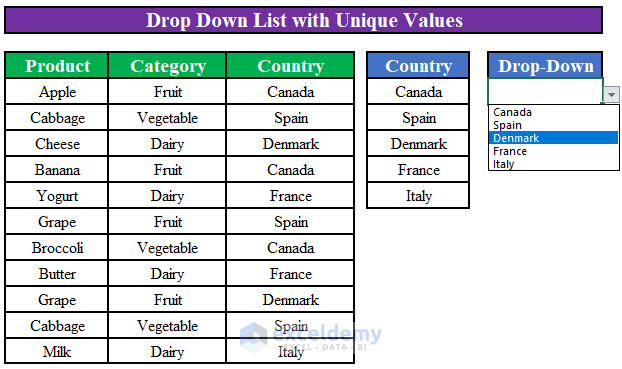
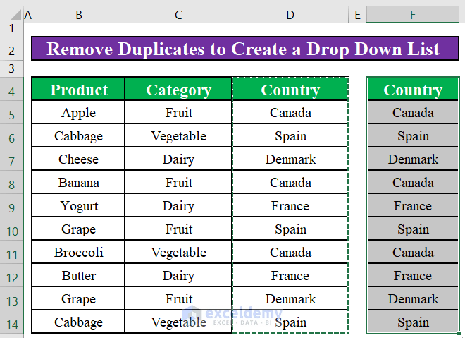
The sample dataset showcases Product name, Category, and Country to which the product is exported.
Method 1 – Insert a Pivot Table to Create a Drop-Down List with Unique Values in Excel
Create a drop-down list with unique values in the Category column:
Step 1:
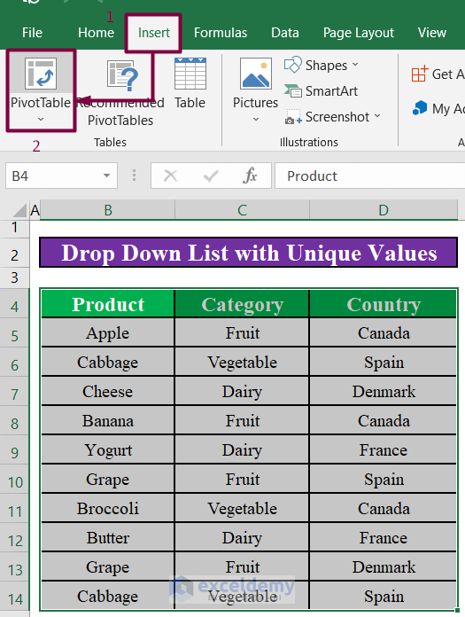
- Select the data range including column headers.
- Click PivotTable in Insert.
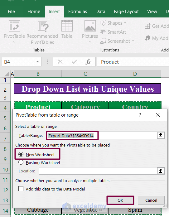
- In the dialog box, data is automatically selected. The default location is a New Worksheet.
- Click OK.
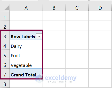
- In PivotTable Fields, drag Category to Rows.
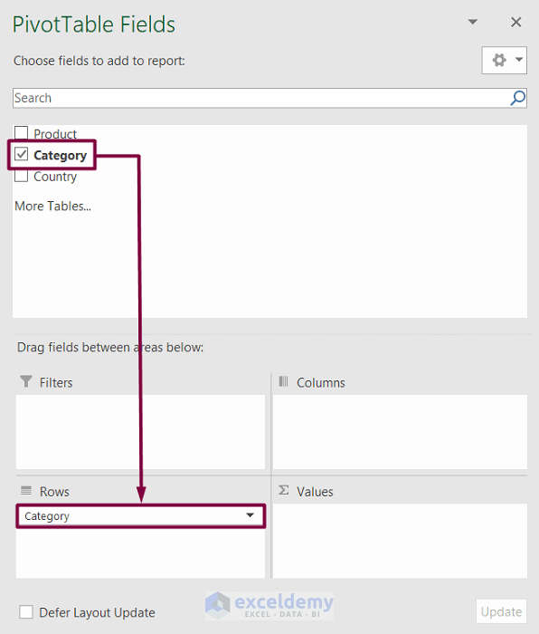
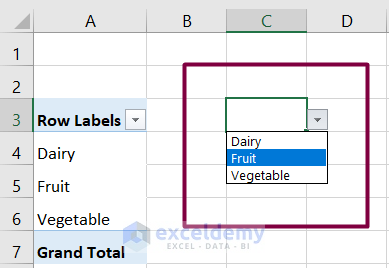
- Excel will create a pivot table:
Step 2:
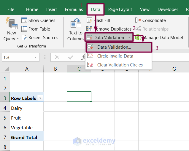
- Select a cell to create a drop-down list. Here, C3.
- Click Data Validation in the Data tab.
- Select Data Validation.
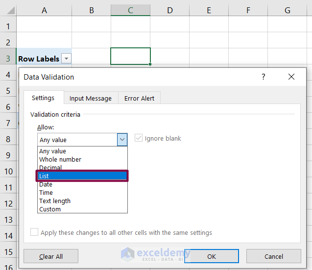
- Select List in Allow.
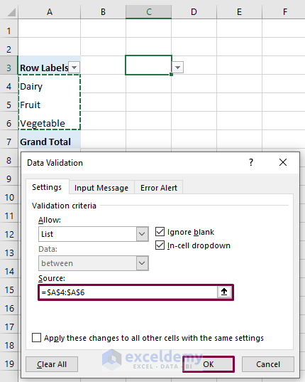
- Enter $A$4:$A$6 in Source.
- Click OK.
You will see a drop-down list in C3 with the unique product categories.
Read More: How to Add Item to Drop-Down List in Excel
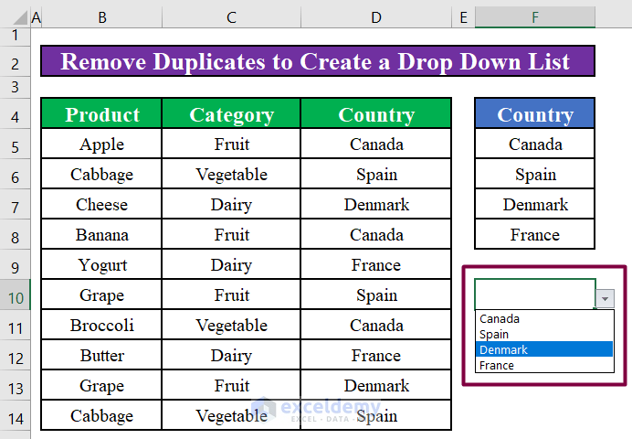
Method 2 – Create a Drop-Down List with Unique Values by Removing Duplicates in Excel
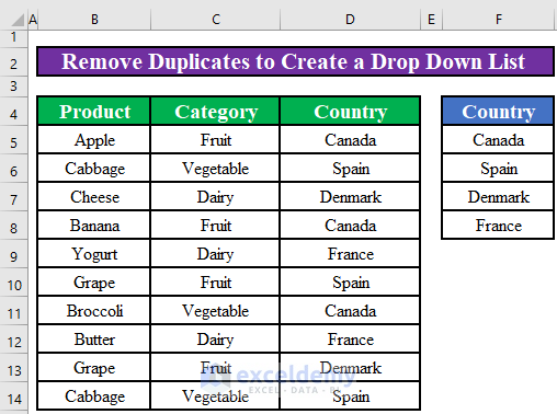
Create a drop-down list with unique values in the Country column:
Step 1:
- Press CTRL+C to copy the cells in the Country column including the column header.
- Paste them into column F pressing CTRL+V.
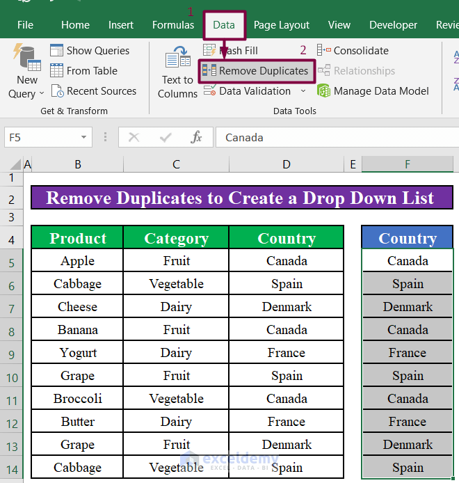
- Select all the cells in Column F.
- Click Remove Duplicates in Data.
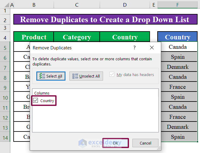
- In Remove Duplicates, the Country is selected in Columns.
- Click OK.
- A box is displayed: 6 duplicate values were found and removed.
- Click OK.
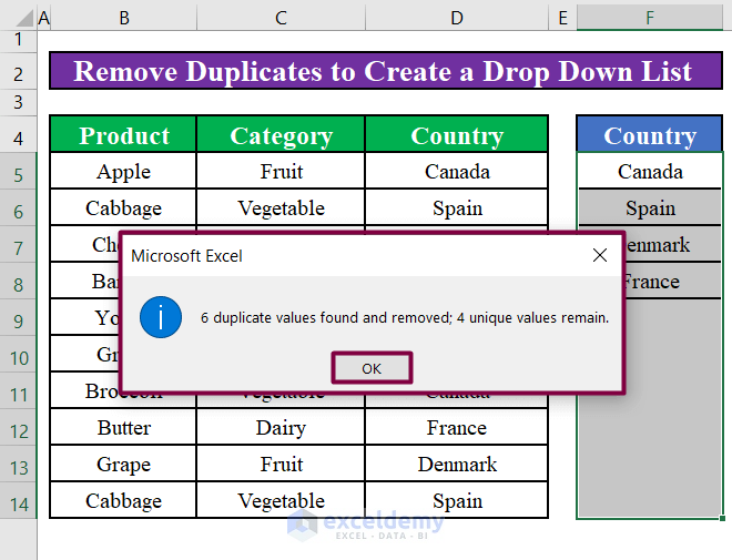
There are 4 unique values.
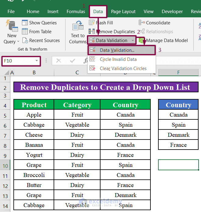
Step 2:
- Select a cell to create the drop-down list. Here, F10.
- Click Data Validation in Data.
- Select Data Validation.
- Select List in Allow.

- Enter $F$5:$F$8 in Source.
- Click OK.
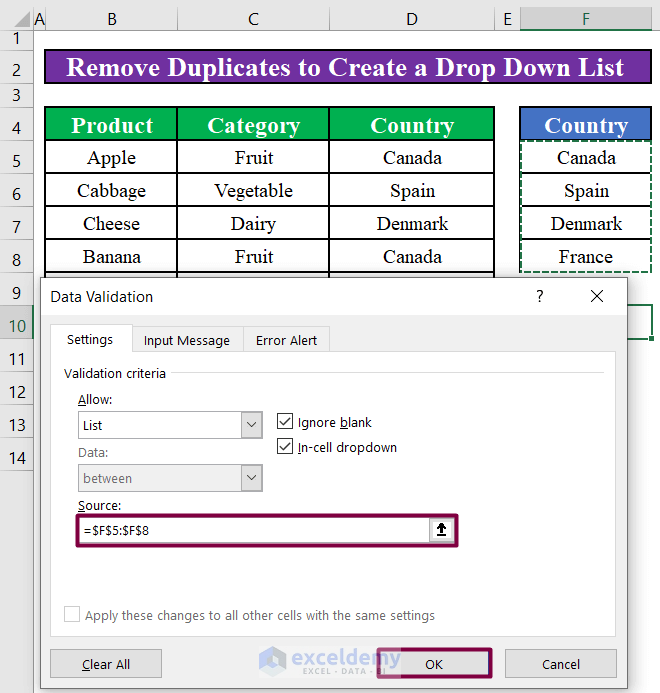
The drop-down list is displayed in F10 with the unique countries.
Read More: How to Remove Duplicates from Drop Down List in Excel
Method 3 – Use the UNIQUE Function to Create a Drop Down List with Unique Values in Excel
Steps:
- Enter the following formula in F5:
=SORT(FILTER(UNIQUE(D5:D14),UNIQUE(D5:D14)<>0))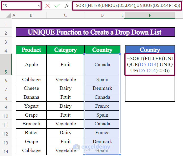
Formula Breakdown:
- The UNIQUE function extracts the unique values in D5:D14.
- The FILTER function returns unique cell values in the Country column that are not null or empty.
- The SORT function sorts the unique values in the Country column in an alphabetical A-Z order.
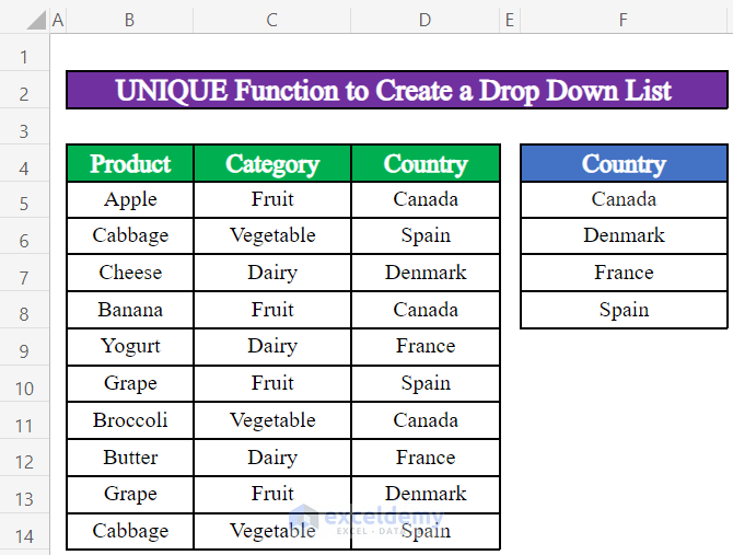
- Press ENTER.
The Country column has 4 unique countries.
- Follow the steps described above to create a drop-down list.
Method 4 – Use a Formula to Create a Dynamic Drop Down List with Unique Values
Steps:
- Follow the steps described above to create a drop-down list.
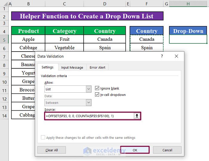
- Select List in Allow.
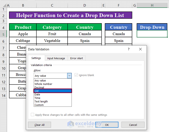
- Enter the following formula in Source:
=OFFSET($F$5, 0, 0, COUNTA($F$5:$F$100), 1)Formula Breakdown:
- The COUNTA function counts the number of cells that are not empty.
- The OFFSET function starts from a specified cell reference, moves down to a specific number of rows, moves right to a specific number of columns, and extracts a section with a specific height and width.
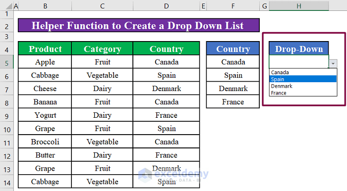
- Click OK.
The drop-down list is displayed in F10 with the unique countries:
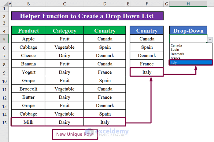
- If you insert a new row with a new country Italy, the drop-down list in H5 automatically updates.
Read More: How to Create a Drop Down List from Another Sheet in Excel
Quick Notes
The UNIQUE function is only available in Excel 365.
Download Practice Workbook
Download the practice book.
Related Articles
- Create Excel Drop Down List from Table
- How to Remove Drop Down List in Excel
- How to Link a Cell Value with a Drop Down List in Excel
- How to Create Excel Drop Down List with Color
- How to Create Drop Down List with Filter in Excel
- How to Copy Filter Drop-Down List in Excel
- Excel Drop Down List Not Working
<< Go Back to Create Drop-Down List in Excel | Excel Drop-Down List | Data Validation in Excel | Learn Excel
Get FREE Advanced Excel Exercises with Solutions!
