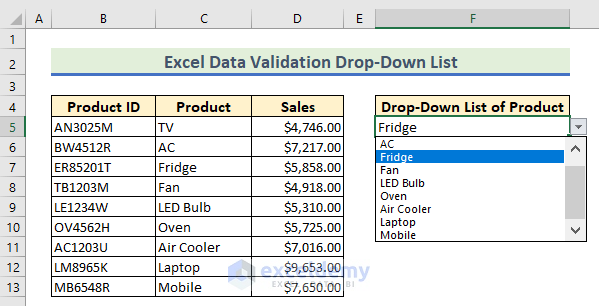
Our dataset contains the sales statements of a company. Using the dataset, we will create a drop-down list in Excel. Here is the overview of our dataset.
What Is Data Validation in Excel?
Data validation allows you to control your input in a cell. When you have limited values to enter a field, you can use the drop-down lists to validate your data. You don’t have to enter data by typing again and again. The data validation list also ensures that your inputs are error-free.
Excel Data Validation Drop-Down List: 5 Practical Examples
Example 1 – Create a Drop-Down List in a Single Cell from Comma Separated Values
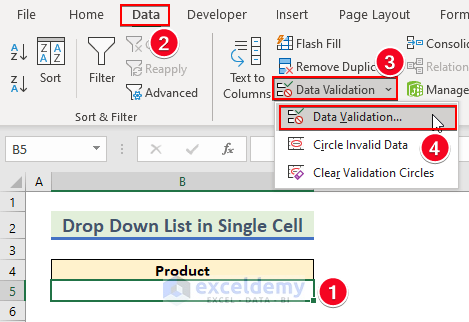
- Select cell B5.
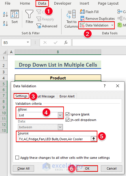
- Go to Data tab.
- From the Data Tools group, select Data Validation and choose Data Validation.
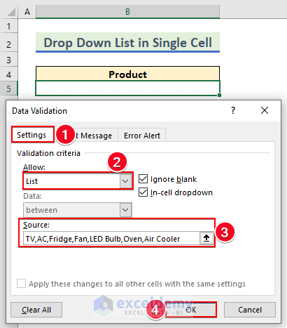
- A Data Validation dialog box pops up. Select the Setting tab.
- Choose List from the Allow drop-down.
- Input the data in the Source typing box that is acceptable to the cell.
- Hit OK.
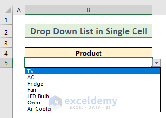
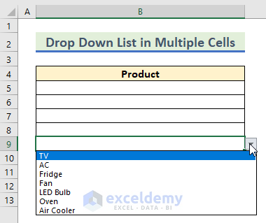
- The list we created is shown here. Click on the data that you want to enter in the cell.
Example 2 – Make Drop-Down Lists in Multiple Cells
- Create a data validation drop-down list like the previous example.
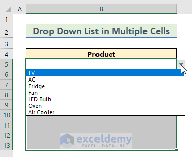
- Drag the AutoFill feature from cell B5 to cell B13 to make a drop-down list in multiple cells.
Alternatively:
- Select all the cells that you want to validate. We selected cells B5 to B13 from our dataset.
- Go to Data Validation and finish the inputs.
- You will be able to create a data validation drop-down list in multiple cells.
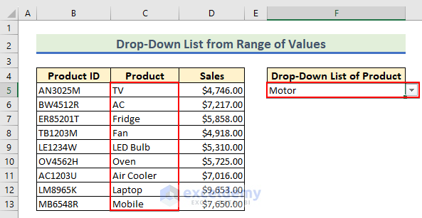
Example 3 – Create a Data Validation Drop-Down List from a Range of Values or a Named Range
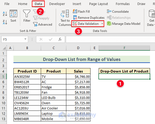
We have a dataset that contains information about several products. The Product ID, Product Name, and Amount of Sales are given in columns B, C, and D.
Case 3.1 – From a Range of Values
- Select cell F5.
- Choose the Data tab.
- From the Data Tools group, select Data Validation.
- A Data Validation dialog box pops up.
- Select the Setting tab.
- Choose List from the Allow drop-down.
- Insert $C$5:$C$13 in the Source box.
- Press OK.
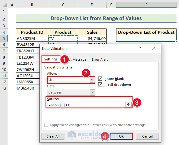
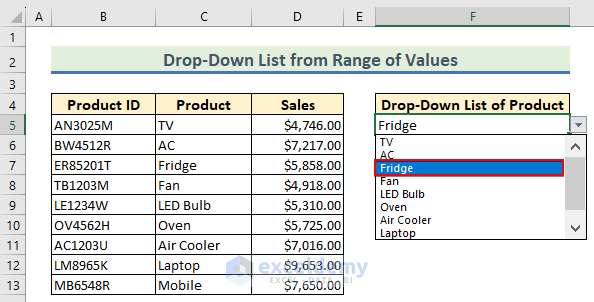
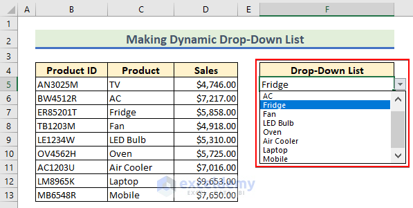
- This creates a data validation drop-down list in Excel from a range of values.
Notes:
If additional data is added to the table after the table itself, the drop-down list will not be updated to include the new data. However, if a cell is inserted within the source data table, any data in that cell will be included in the drop-down list.
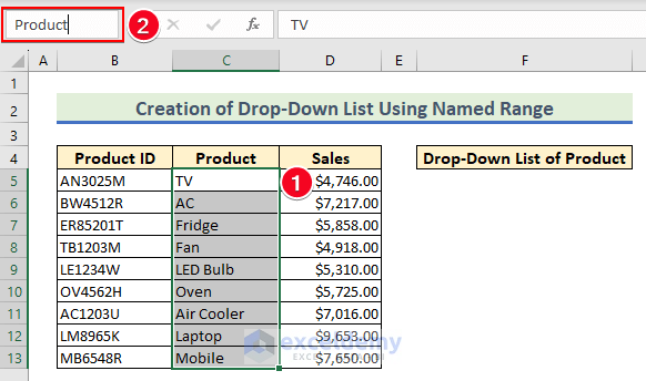
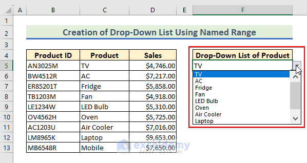
Case 3.2 – Using a Named Range
- Select cells C5 to C13 and name this range as Product.
- Select the cell where you need the drop-down and open Data Validation.
- Use the following formula in the Source typing box of the Data Validation dialog box.
=Product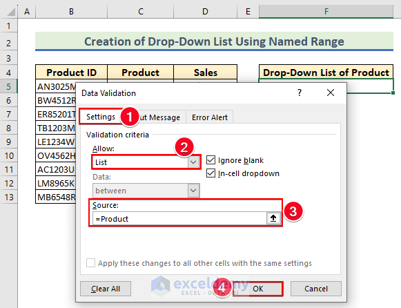
- The drop-down list will be created using the Named range.
Read More: How to Make a Data Validation List from Table in Excel
Example 4 – Use a List to Make a Data Validation Drop-Down List
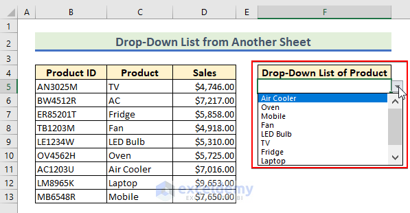
Case 4.1 – From Another Sheet
- We have used a list from a different sheet named List. And in the Source field, you can see the sheet name and the cell references.
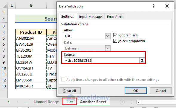
- The final output is given in the below screenshot.
Read More: How to Use Data Validation List from Another Sheet
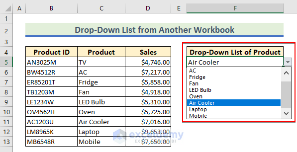
Case 4.2 – From Another Workbook
- Use the following formula in the Source field in the Data Validation dialog box, then press OK.
=INDIRECT("'[Source Data.xlsx]Named Range'!Product")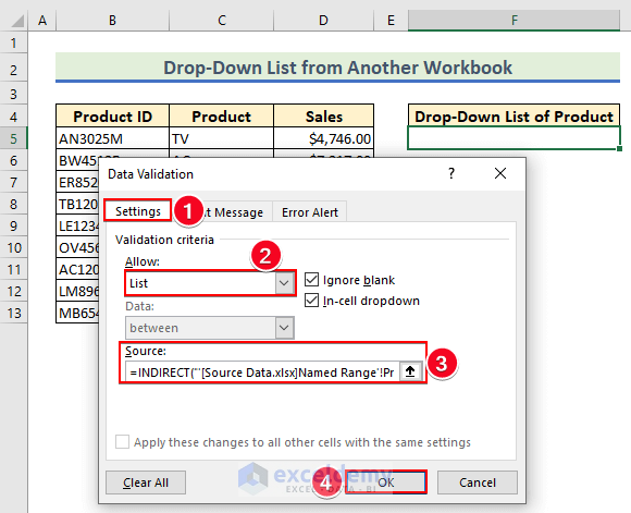
Formula Breakdown
=INDIRECT(“‘[Source Data.xlsx]Named Range’!Product”)
- Product is the named range of cells that you have entered into the drop-down list.
- Named Range: This tells Excel to look for the named range on a sheet named Named Range.
- [Source Data.xlsx] which tells Excel to look for the named range in a workbook named “Source Data.xlsx“.
- The INDIRECT function returns the value of the reference specified by a text string.
Notes:
The workbook which contains the source data must be open in order for the drop-down list to work. If the other workbook is closed, the drop-down list will display an error message
Example 5 – Make a Searchable / Dynamic / Dependent or Conditional Drop-Down List in Excel
Case 5.1 – Searchable Drop-Down List
- Insert the following formula in cell E5 in the sheet named SalesInfo.
=FILTER(B5:B13,ISNUMBER(SEARCH(Searchable!B4,B5:B13)),"Not Found")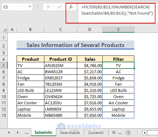
Formula Breakdown
- The SEARCH function in the formula searches for a given value.
- The ISNUMBER function returns True if the output of the SEARCH function is a number. Otherwise, it returns False.
- The FILTER function filters data according to the given criteria.
- Select cell B4 in the Searchable worksheet.
- Select Data Validation.
- Choose List from the Allow: field.
- Enter the following formula in the Source field.
=SalesInfo!$E$5#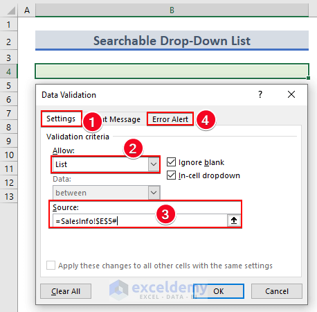
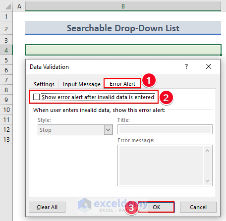
- Go to the Error Alert tab.
- Uncheck Show error alert after invalid data is entered.
- Press OK.
- A searchable drop-down list has been created.
- Type something (F) in cell B4.
- Select the dropdown arrow visible at the lower right corner of the cell.
- You will see all the relevant search results as shown in the following picture.

Read More: Excel Data Validation Drop Down List with Filter
Case 5.2 – Dynamic Drop-Down List
- In the source field, apply the following formula.
=OFFSET($C$5,0,0,COUNTIF($C$5:$C$100,"<>"))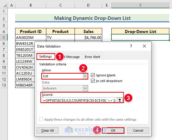
Formula Breakdown
=OFFSET($C$5,0,0,COUNTIF($C$5:$C$100,”<>”))
- COUNTIF($C$5:$C$100,”<>”) is the [height] of the OFFSET function which counts the non-blank cells in the range C4:C100.
- 1st and 2nd 0 are the Rows and Columns.
- $C$5 is the Reference of the COUNTIF function.
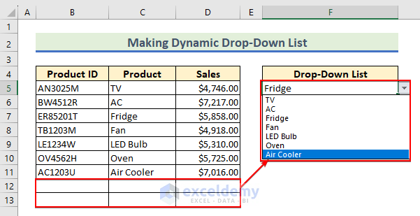
- Delete some data from your data list, and the drop-down list automatically updates itself.
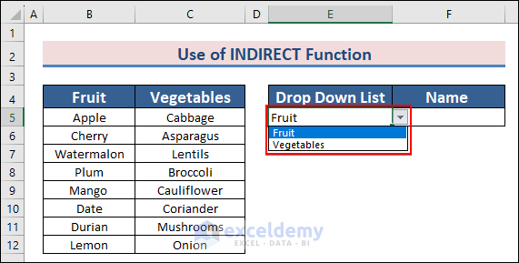
Case 5.3 – Dependent or Conditional Drop-Down List
- Create a drop-down list from the column header range.
- Click OK to continue.
- We have our drop-down list for the columns.
- Select the Fruit and Vegetable column, go to Formulas and in the Name Manager, click on Create From Selection.
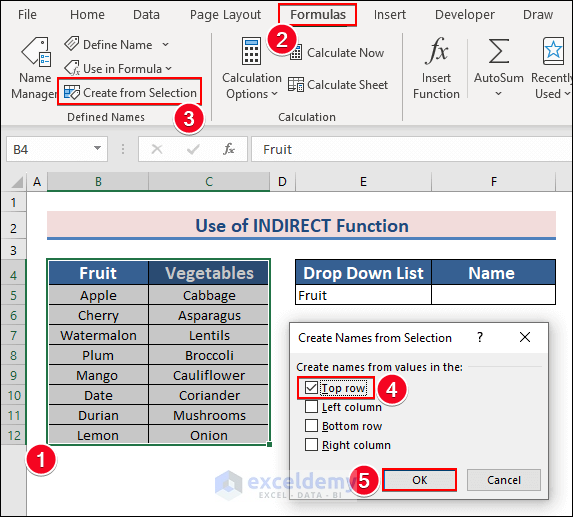
- Check Top Row and click OK.
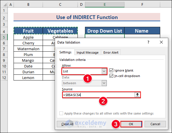
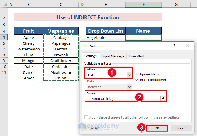
- Select cell F4 and go to Data Validation.
- Select List.
- In the Source box, apply this formula:
=INDIRECT(E5)When you select Fruit in the drop-down list (E4), this refers to the named range Fruit (through the INDIRECT function) lists all the items in that category.
- Click OK.
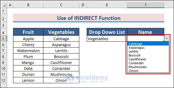
- If you change Fruit to Vegetables, the list will show you the vegetable names.
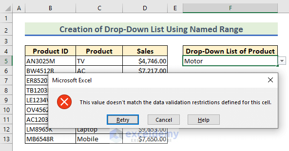
How to Handle Errors in a Data Validation Drop-Down List
While inserting any item that is not on our list, Excel shows an error. We will insert Motor and press Enter. You will see the following message:
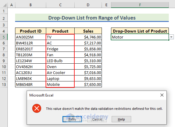
As our item was not on the list, it won’t take this as a valid item. This is an Error Alert in data validation. You can customize it in various ways.
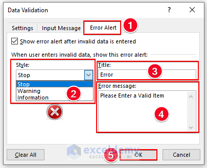
In Microsoft Excel, you can show three types of error messages. These are Stop, Warning, and Information.
Select the Title and Error Message you want to show when a user gives an invalid input. Press OK.
Case 1 – Stop Style Error
It will appear when the user gives an invalid entry. This option allows the user to retype or cancel the attempt.

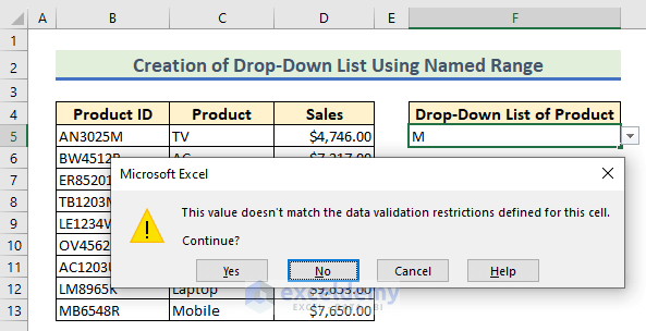
Case 2 – Warning Style Error
The warning style shows a message that gives a user a choice to allow the item that is not in the list you selected.
Case 3 – Information Style Error
The Information style shows a message that automatically authorizes the item no matter what the user gave. It shows the user the data validation rules.

How to Allow Entries That Are Not in Excel Drop-Down List
Method 1 – Turn Off Error Checking
To allow entries that are not on the list, you can turn off the error-checking option. By doing that, Excel won’t show any error message for other values and it will accept any item given by the user.
- In the Data Validation dialog box, select the Error Alert tab.
- Uncheck the first box.
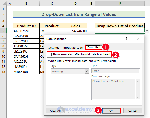
- You can enter any other values outside the list in the Excel data validation list.
Method 2 – Choose Other Error Alerts Options
Another useful way to allow other entries is to choose different error alert options. We have already shown you different types of error alerts. According to that, choose the Information style.
This error alert allows you to enter different items in the column.
How to Remove a Drop-Down List in Excel
- Select the drop-down cell .
- Choose the Data tab.
- Select the Data Validation feature.
- From the Data Validation dialog box, select Clear All and hit OK.
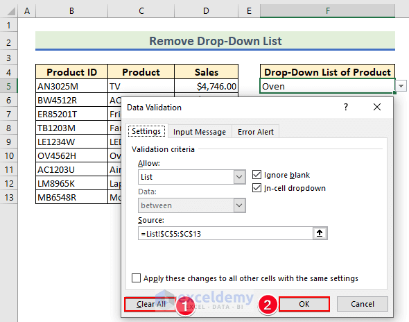
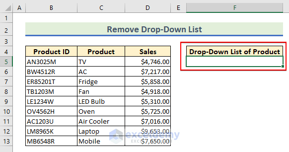
- This removes the drop-down list.
Benefits of Using Data Validation Drop-Down List
- Reduces errors: By restricting the entries in a cell to a predefined set of values, the Data Validation Drop-Down List reduces the chances of errors in data entry.
- Saves time: The drop-down list makes data entry faster and more efficient, as users can select a value from the list instead of typing it manually.
- Consistency: The Data Validation Drop-down List ensures that the data entered in a cell is consistent and conforms to the predefined set of values.
- Flexibility: You can easily modify the list of values in the drop-down list as needed, without affecting the existing data
Things to Remember
- You can copy any cell with data validation and paste it into other cells. The resulting cells will have the same drop-down list.
- Use a separate sheet to store the list of values that you want to appear in the drop-down list. This makes it easier to manage and update the list of values.
- Use named ranges to define the list of values. This makes it easier to reference the list of values in other parts of the workbook.
- Consider using data validation for other types of data, such as dates or times. This can help to ensure that the data entered in the cell is valid and consistent.
Frequently Asked Questions
How do I make a drop-down list dependent on another drop-down list?
To make a drop-down list dependent on another drop-down list, use named ranges and the INDIRECT function. Create two named ranges, one for the first list and one for the second list, and use the INDIRECT function in the Source box of the second list to reference the first list based on its value.
How do I prevent users from entering data that is not in the drop-down list?
To prevent users from entering data that is not in the drop-down list, go to the Data tab, click on Data Validation, select List from the Allow drop-down menu, and make sure to check the box next to In-cell dropdown and Ignore blank. This will limit user input to the values in the drop-down list.
Is a drop-down list equivalent to data filtering?
No, a drop-down list and data filtering are not the same. A drop-down list allows the user to select a value from a predefined list of options, while data filtering allows the user to narrow down a larger set of data based on specific criteria. Both can be used to facilitate data entry and analysis in Excel, but they serve different purposes.
Download the Practice Workbook
Related Articles
<< Go Back to Create Drop-Down List in Excel | Excel Drop-Down List | Data Validation in Excel | Learn Excel
Get FREE Advanced Excel Exercises with Solutions!

Category Item Avg Sale Price
Tablet ACER 4000
Tablet DELL 10000
Tablet HP 1500
Hardware Mouse 150
Hardware Keyboard 600
Hardware Webcam 1200
This is table and now want to dropdowns over category and item accordingly once i am selecting Tablet so i only want items related to Teblet like Acer, Dell HP
Hello Akash Mathur,
To create dependent drop-downs (also called cascading drop-down lists) in Excel—so that selecting “Tablet” in the Category drop-down shows only related items (Acer, Dell, HP) in the Item drop-down—you can use named ranges and Data Validation with the INDIRECT function.
Steps to do it:
1. Create a unique list for Categories (e.g., Tablet, Hardware).
2. Create separate lists for each category’s items (e.g., a list of Tablet items: Acer, Dell, HP).
3. Name each item list exactly as the Category (e.g., name the Tablet items range “Tablet”).
4. Add Data Validation to the Category cell with the category list as the source.
5. Add Data Validation to the Item cell with the formula =INDIRECT(CategoryCell) as the source (replace CategoryCell with the actual cell reference).
Now, when you pick “Tablet” in the Category drop-down, only Acer, Dell, and HP will be available in the Item drop-down.
We also have other articles regarding dependent dropdown, you can explore these articles:
How to Create a Dynamic Dependent Drop-Down List in Excel
Excel Dependent Drop Down List (Create with Easy Steps)
Regards
ExcelDemy