How to Make a Data Validation List from Table in Excel (3 Methods)

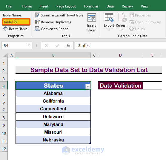
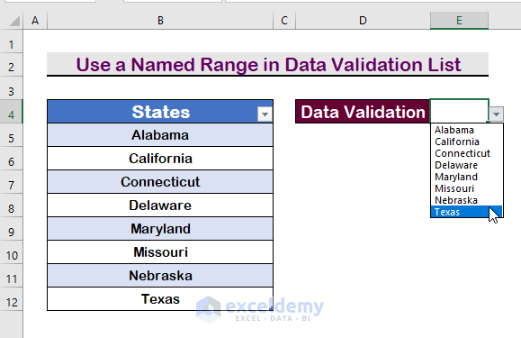
Here’s a sample data set to use for the validation list.

• We opened the Data Validation option from the Data tab.

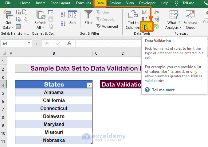
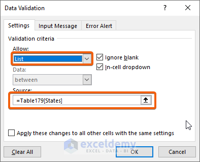
• We selected the List option as Allow and type the table name with the header (Table179[States]).

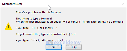
• But it didn’t work and we got an error message. Let’s see how to solve this.

Method 1 – Apply Cell References in the Data Validation List from a Table in Excel

Steps:

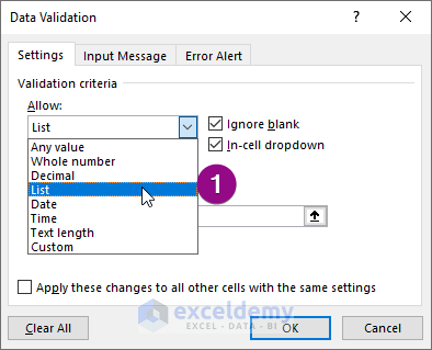
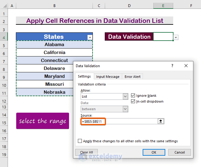
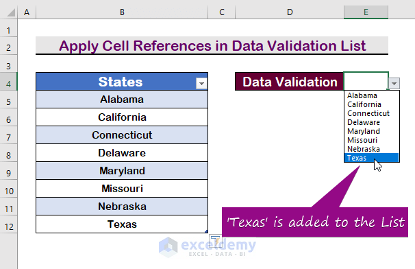
• Go to the Data tab and select Data Validation.
• Select List under Allow.

• In the Source box, select the range B5:B11 without its header
• Press Enter.

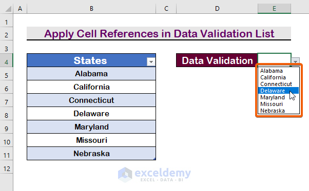
• Your Data Validation drop-down list will appear.

• Type an extra element ‘Texas’ at the bottom of the table.

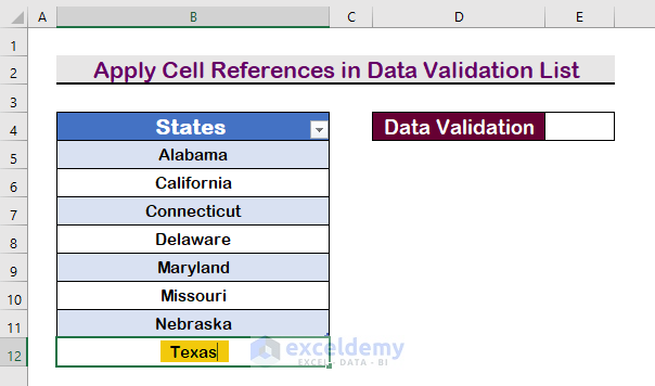
• The new element ‘Texas’ is added to the Data Validation

Read More: Excel Data Validation Drop-Down List

Method 2 – Use a Named Range in a Data Validation List from a Table in Excel

Steps:

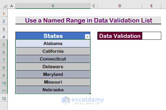
• Select the cells in the range without the Table Header.

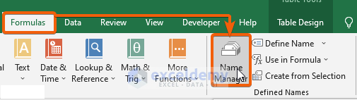
• Click on the Formulas tab.
• Click on Name Manager.

• Click on New.

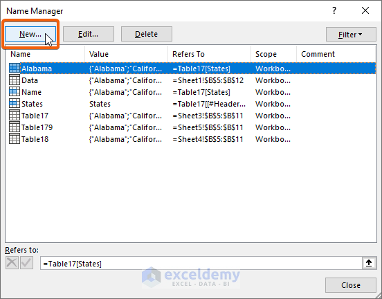
• Type any name. We chose Named_Range.
• Press Enter.

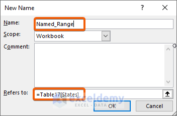
• In the Data Validation Source box, insert that name after an equals sign.

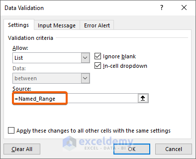
• Press Enter to see the list.

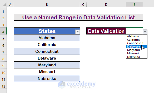
• Add a value to the bottom of the range.

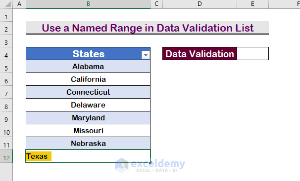
• The new value will be added to the drop-down option.

Read More: Excel Data Validation Drop Down List with Filter

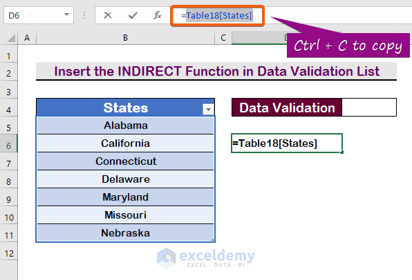
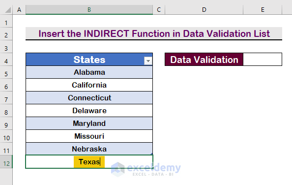
Method 3 – Insert the INDIRECT Function in the Data Validation List

Steps:

• In any cell, type the ‘=’ equals sign and select the range.
• Copy the range name Table18[States].

• In Data Validation, use the following formula with the INDIRECT function:

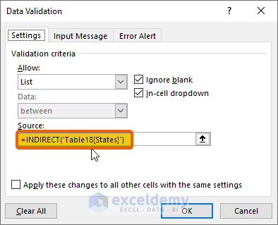
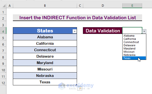
• Press Enter to see the list.

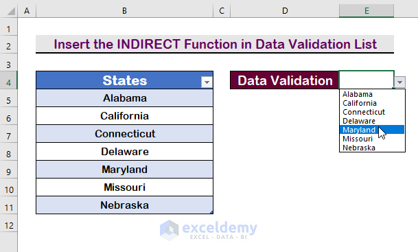
• Insert a value at the bottom of the table.

• It will be added to the Data Validation list automatically.

Download the Practice Workbook

Related Articles

• How to Use Data Validation List from Another Sheet
• How to Set Limit in Excel Cell
• How to Use Excel Formula Not to Exceed a Certain Value

<< Go Back to Data Validation in Excel | Learn Excel