Method 1 – Using the OFFSET Function
Steps:
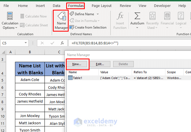
- Enter the following formula in cell C5:
=FILTER(B5:B14,B5:B14<>"")
Here, the FILTER function will take the range B5:B14 and check any blanks between the range. It filters out empty or blank cells from the list.
- Press the ENTER. You will see the list of names without any blanks.
![]()
- Select Name Manager from the Formula Tab and click New.
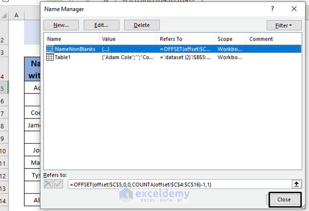
- Give your range a name. (i.e., NameNonBlanks)
- Enter the following formula in Refers to:
=offset(offset!$C$5,0,0,counta(offset!$C$4:$C$16)-1,1)![]()
- Click OK. You will see a Window. Close it.
- Select cell D5 and select Data >> Data Validation List.
- Change the Source Name to =NameNonBlanks.
- Click OK.
![]()
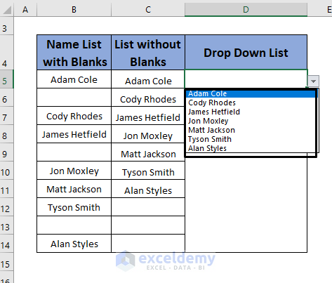
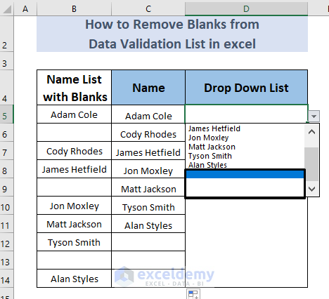
- Select the drop-down list bar in cell D5. You will see the list of names we are using.
- Enter some new names throughout cells C12 to C16.
- Then select the data validation list in cell D5.
![]()
The new names are in your drop-down list. However, you can’t see any new entries under cell C16 because they are outside your range.
Read More: How to Use Custom VLOOKUP Formula in Excel Data Validation
Method 2 – Using the Go to Special Command
Steps:
- Select the cells B5 to B14 and select Home >> Find & Select >> Go To Special.
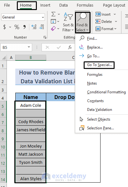
- Select Blanks and click OK.
![]()
This operation will select the blank cells.
- Select any of these blank cells, right-click on it, and select Delete to delete the blanks.
![]()
- You will see a dialog box. Select Shift cells up and click OK.

This operation will remove the blanks from the original list as well as from the drop-down list.
![]()
Method 3 – Using the Excel Filter Function
Steps:
- Enter the following formula in cell C5:
=FILTER(B5:B14,B5:B14<>"")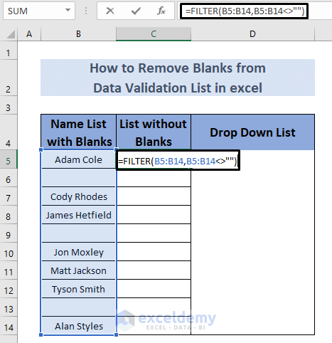
The FILTER function will take the range B5:B14 and check any blanks between the range. It filters out empty or blank cells from the list.
- Press the ENTER key to see the list of names without any blanks.
![]()
- If you go to the Drop-Down List, you will still see that it contains blanks from column C.

- To remove these blanks, go to Data Validation from Data Tab.
- Change the final cell of the range to C11, as your filtered list has the range C5 to C11 in the Source.
![]()
- Click OK. You will now have no blank cells in your drop-down list.

Method 4 – Combining IF, COUNTIF, ROW, INDEX and Small Functions
Steps:
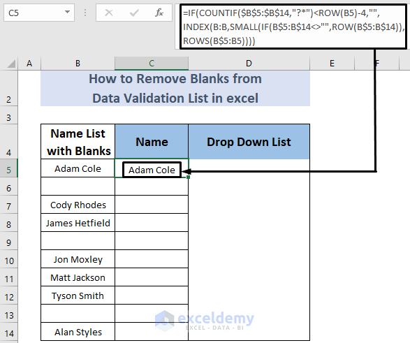
- Enter the following formula in cell C5:
=IF(COUNTIF($B$5:$B$14,"?*")<ROW(B5)-4,"",INDEX(B:B,SMALL(IF(B$5:B$14<>"",ROW(B$5:B$14)),ROWS(B$5:B5))))![]()
Formula Breakdwon
The formula has two main parts. The first part is COUNTIF($B$5:$B$14,”?*”)<ROW(B5)-4,”” and the second one is INDEX(B:B,SMALL(IF(B$5:B$14<>””,ROW(B$5:B$14)),ROWS(B$5:B5))).
- The COUNTIF function counts non-blank text here and that’s why we get the 7 names in column C.
- The ROW function returns the row number of a cell and our empty cell is at position 5 from cell B5. We are subtracting 4 because we want it to be less than that.
- Press enter.
- Use the Fill Handle to AutoFill the lower cells.
![]()
- We have the Name list without any blanks. But if we click on the data validation list, we still see blanks in the drop-down list.
- To remove these blanks, go to Data Validation from the Data Tab.
- Change the final cell of the range to C11, as your filtered list has the range C5 to C11 in the Source.
![]()
- Click OK. You will now have no blank cells in your drop-down list.

Read More: How to Use IF Statement in Data Validation Formula in Excel
Method 5 – Utilizing Combined Functions
Steps:
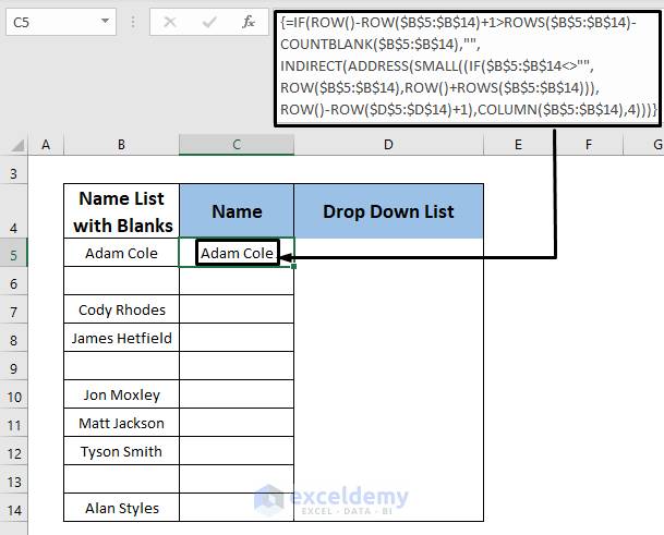
- Enter the following formula in cell C5:
=IF(ROW()-ROW($B$5:$B$14)+1>ROWS($B$5:$B$14)-COUNTBLANK($B$5:$B$14),"", INDIRECT(ADDRESS(SMALL((IF($B$5:$B$14<>"",ROW($B$5:$B$14),ROW()+ROWS($B$5:$B$14))),ROW()-ROW($C$5:$C$14)+1),COLUMN($B$5:$B$14),4)))![]()
Here, I’ll explain how this formula works in a very simple way. It goes through the range B5:B14 and checks the blank cells with the help of the COUNTBLANK function. Then, it also checks which cells are not blank throughout B5:B14, and thus, it returns non-empty cells.
- Press CTRL + SHIFT + ENTER (because it’s an array formula), and you will see the output in cell C5 below.
- Use the Fill Handle to AutoFill the lower cells.
![]()
- If you go to the Drop-Down List, you will still see that it contains blanks from column C.
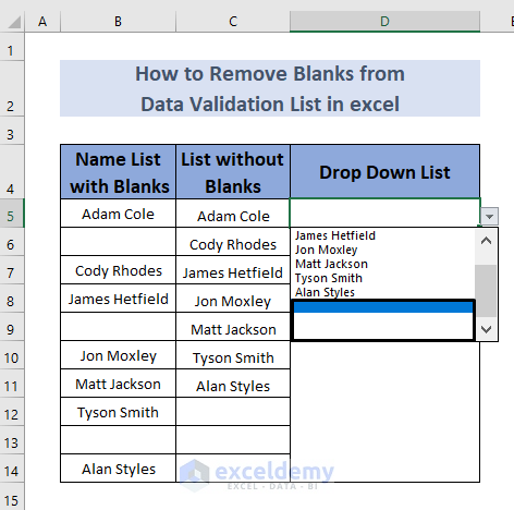
- To remove these blanks, go to Data Validation from the Data Tab.
- Change the final cell of the range to C11, as your filtered list has the range C5 to C11 in the Source.
![]()
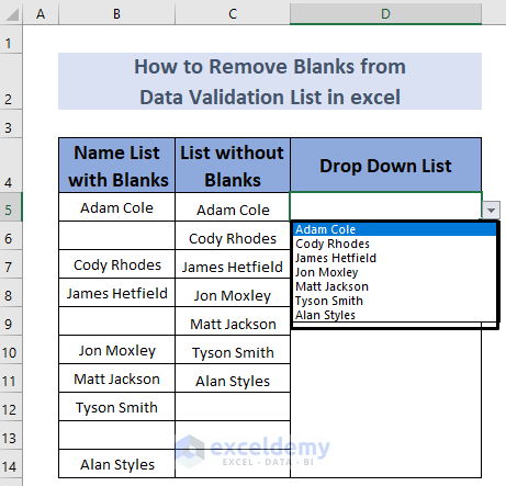
- Click OK. You will now have no blank cells in your drop-down list.
Read More: How to Remove Data Validation Restrictions in Excel
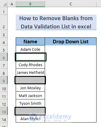
Practice Section
Here is the dataset so that you can practice these methods on your own.
![]()
Download the Practice Workbook
Related Articles
- Apply Custom Data Validation for Multiple Criteria in Excel
- How to Apply Multiple Data Validation in One Cell in Excel
- Data Validation Based on Another Cell in Excel
- How to Copy Data Validation in Excel
<< Go Back to Data Validation in Excel | Learn Excel
Get FREE Advanced Excel Exercises with Solutions!
