In this article we’ll discuss how to use Custom Data Validation with multiple criteria to prevent incorrect or out-of-range data being entered into a worksheet.
Example 1 – Apply Custom Data Validation for Multiple Criteria in One Excel Cell
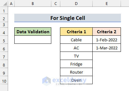
Consider the following dataset, which has two criteria for data being input: Criteria 1 contains a list of products, and Criteria 2 contains 2 specific dates. Let’s apply Data Validation using the OR function to restrict input in cell B5 to data matching either of the 2 criteria. The OR function returns TRUE if any of the arguments or conditions in the argument are met, and FALSE if not.
STEPS:
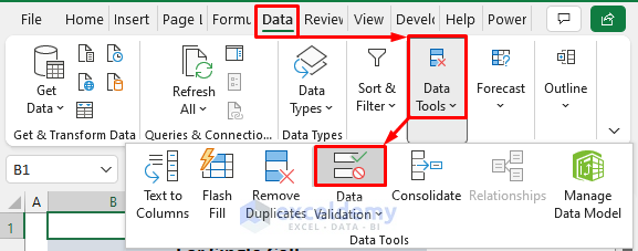
- Under the Data tab, select Data Validation from the Data Tools group.
The Data Validation dialog box will pop out.
- Under the Settings tab, select Custom in the field Allow.
- In the Formula box, enter the formula:
=OR(COUNTIF($D$5:$D$10,B5)=1, AND(B5>=E5,B5<=E6))- Click OK.
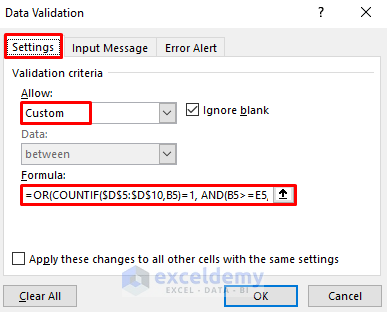
Here, the AND function checks whether the date input is between E5 (1-Feb-2022) & E6 (1-Mar-2022). The COUNTIF function checks if the B5 text value has a match in the range D5:D10. Finally, the OR function checks if the value in B5 satisfies either of the specified conditions.
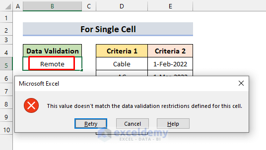
- Enter any of the products from Criteria 1 or any date between the specified dates.
If you enter anything that doesn’t comply with either of the conditions, you’ll get an error dialog box.
Read More: How to Apply Multiple Data Validation in One Cell in Excel
Example 2 – Use Custom Data Validation for Multiple Criteria in Selected Cells
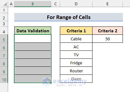
We can apply Data Validation in a range of cells instead of just a single cell as in the previous example. In the below dataset, we have 2 criteria: Criteria 1 has a list of products, and Criteria 2 has a number input which is 50.
Let’s restrict input to either of our specified criteria in the range B5:B10.
STEPS:
- Select the range B5:B10.
- Go to Data ➤ Data Tools ➤ Data Validation.
The Data Validation dialog box will pop out.
- Under the Settings tab, select Custom in the Allow field, and in the Formula box, enter:
=OR(B5<$E$5,COUNTIF($D$5:$D$10,B5)=1)- Press OK.
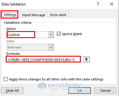
The COUNTIF function checks whether the input is in the range D5:D10. The other criterion is that the input is smaller than E5 (50). Then the OR function checks if the inputs in the range B5:B10 satisfy any of the conditions.
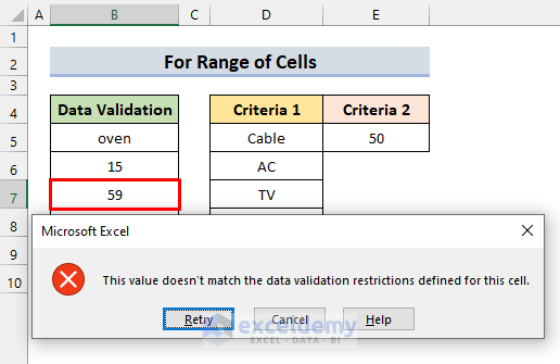
- Input some valid data that satisfies the conditions.
In this example, “oven” and “15” in cells B5 and B6 are valid. But, if we try to input “59”, an error message will be returned, as 59 is greater than 50.
Example 3 – Prevent Duplicate Entries and Limit the Number of Characters with Custom Data Validation
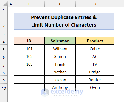
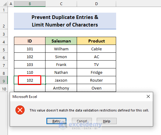
The below dataset represents the ID, Salesman, and Product of a company. Some IDs are missing. Let’s complete the list of IDs, only allowing unique numbers of 3 digit length.
STEPS:
- Select the range B5:B10.
- Go to Data ➤ Data Tools ➤ Data Validation.
A dialog box will appear.
- Under the Settings tab, select Custom in Allow.
- In the Formula box, enter the formula:
=AND(COUNTIF($B$5:$B$10,B5)<=1, ISNUMBER(B5), LEN(B5)=3)- Press OK.
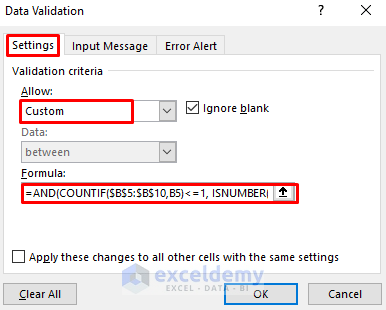
The ISNUMBER function takes number inputs. The LEN function checks that the input is only 3 digits long. The COUNTIF function prevents any duplicate entries. Then the AND function checks whether the entries satisfy all the conditions or not. An entry will be valid only if the entries satisfy all the conditions.
- Input any valid data maintaining all the criteria.
Invalid data (like a duplicate value) will result in an error dialog box.
Read More: How to Remove Data Validation Restrictions in Excel
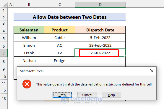
Example 4 – Allow Dates between Two Dates with Custom Data Validation
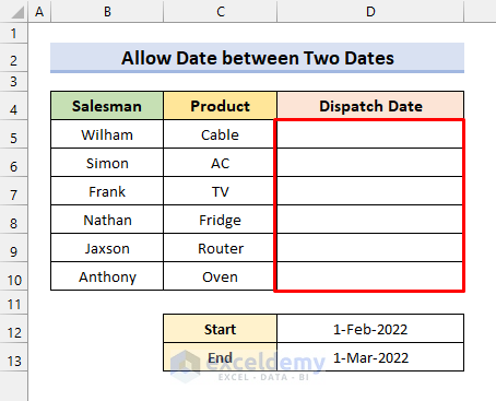
In the following dataset, we have a start date in cell D12 and an end date in cell D13. Let’s use Custom Data Validation to only allow date entries between the two given dates in the Dispatch Date column.
STEPS:
- Select the range D5:D10.
- Select Data ➤ Data Tools ➤ Data Validation.
The Data Validation dialog box will pop out.
- Under the Settings tab, select Custom in the Allow field.
- In the Formula box, enter:
=AND(D5>=$D$12, D5<=$D$13)- Click OK.
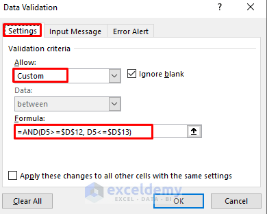
Here, the AND function checks whether the date entries fall between the dates in cells D12 and D13.
You’ll be able to input dates following the criterion. But as soon as you type any invalid date that doesn’t satisfy the condition, you’ll get an error message.
In this example, although “29-02-2022” falls within the specified dates, an error box is returned, because 2022 is not a leap year and thus 29th February doesn’t exist.
Download Practice Workbook
Related Articles
- How to Use IF Statement in Data Validation Formula in Excel
- How to Use Custom VLOOKUP Formula in Excel Data Validation
- Data Validation Based on Another Cell in Excel
- How to Copy Data Validation in Excel
- How to Remove Blanks from Data Validation List in Excel
<< Go Back to Excel Custom Data Validation | Data Validation in Excel | Learn Excel
Get FREE Advanced Excel Exercises with Solutions!

I would like to create a spreadsheet for our three companies. When choosing the company, I am looking to have the tables listed for that company. Is this possible? I have been trying to understand the steps to work this out but not finding what I am looking for.
Hi Jenn,
Based on your comment, it seems you are looking for a way to create a spreadsheet that displays different tables based on the selected company.
To address your requirement, one approach is to use Excel’s “Data Validation” feature combined with “Index” and “Offset” functions. Here’s a potential step-by-step solution:
1. Set up your spreadsheet with separate tables for each company, each in a different range of cells.
2. Create a list of company names (e.g., in a dropdown) where the user can select the desired company.
3. Assign data validation to the cell where the user selects the company, limiting the input to the list of company names.
4. Next, use the “Index” and “Offset” functions to display the corresponding table based on the selected company.
Here’s an example of how this could work:
1. Create separate tables for each company, each in a different range of cells (e.g., Company A in cells A1:D10, Company B in cells A15:D24, Company C in cells A29:D38).
2. Create a dropdown list of company names (e.g., in cell A50) using Excel’s Data Validation feature.
3. Use the “Index” and “Offset” functions to retrieve the appropriate table based on the selected company. For example, in cell A55, you could use the following formula:
=INDEX($A$1:$D$10, OFFSET($A$1:$A$10, MATCH($A$50,$A$1:$A$10,0)-1, 0, ROWS($A$1:$A$10), COLUMNS($A$1:$D$10)))This formula will retrieve the table for the selected company dynamically.
Now, when you select a company from the dropdown list in cell A50, the corresponding table will be displayed in cell A55 and automatically update based on the selection.
Please note that the specific ranges and formulas may need to be adjusted based on the actual structure and layout of the spreadsheet. However, this approach should provide a starting point to achieve the desired functionality of displaying different tables based on the selected company in Excel.
Regards,
ExcelDemy