Data Validation Based on Another Cell in Excel (4 Examples)

How to Do Data Validation in Excel?

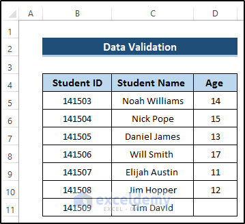
Take a dataset that includes student ID, student name, and age. We would like to make a data validation where the age must be less than 18.

Select cell D11.
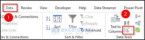
Go to the Data tab on the ribbon.
Select the Data validation drop-down option from the Data Tools group.

As a result, the Data Validation dialog box will appear.

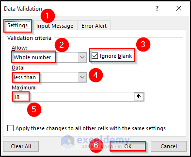
Select the Settings tab.
Select the Whole Number option from the Allow section.
Check on the Ignore Blank option.
Select the less than option from Data.
Set the Maximum value to 18.
Click on OK.

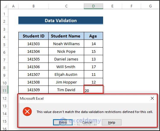
Next, if we write 20 as age, it will show an error because it is above our maximum limit in the data validation. That’s what we get from data validation.

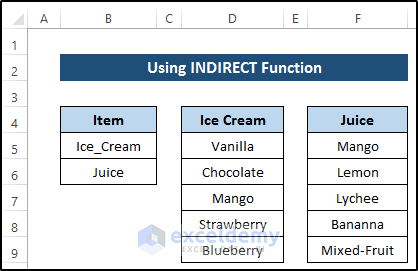
Method 1 – Applying INDIRECT Function

Let’s take a dataset that includes two items and their different types.

Steps

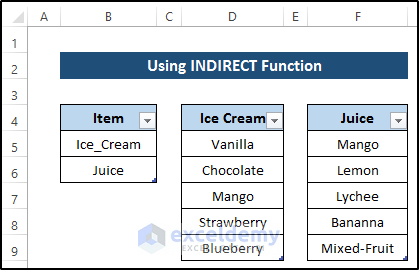
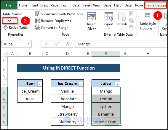
Convert all three columns into different tables.

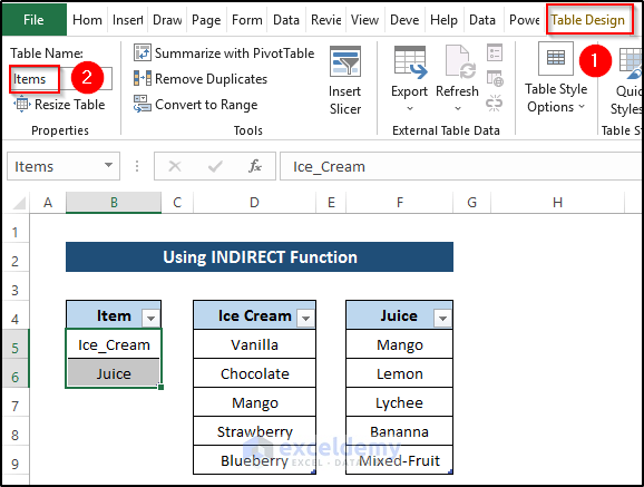
Select the range of cells B5 to B6.
The Table Design tab will appear.
Go to the Table Design tab on the ribbon.
Change the Table Name from the Properties group.

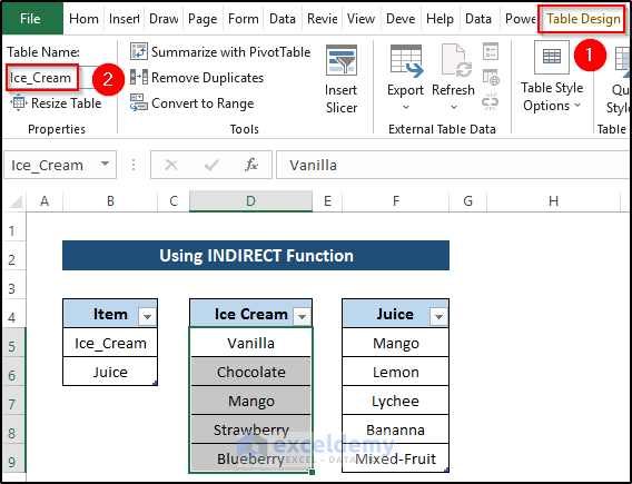
Select the range of cells D5 to D9.
Change the Table Name from the Properties group.

Select the range of cells F5 to F9.
Change the Table Name from the Properties group.

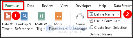
Go to the Formula tab on the ribbon.
Select Define Name from the Define Names group.

The New Name dialog box will appear. Set the name.
In the Refers to section, write down the following:

=Items[Item]

Click on OK.
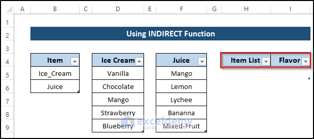
Create two new columns to add data validation.
Select cell H5.

Go to the Data tab on the ribbon.
Select the Data Validation drop-down option from the Data Tools group.

The Data Validation dialog box will appear.
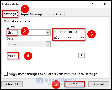
Select the Settings tab on the top.
Select List from the Allow options.
Check on the Ignore blank and In-cell dropdown options.
Write down the following in the Source section:

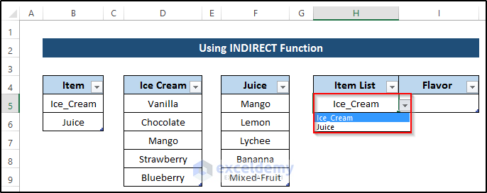
=Item

Click on OK.

You will get the following drop-down option where you can select either ice cream or juice.

Select cell I5.
Go to the Data tab on the ribbon.
Select the Data Validation drop-down option from the Data Tools group.

The Data Validation dialog box will appear.
Select the Settings tab on the top.
Select List from the Allow section.
Check the Ignore blank and In-cell dropdown options.
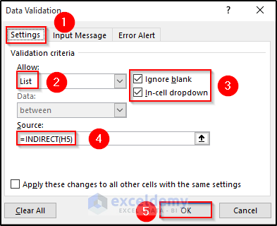
Write down the following in the Source section:

=INDIRECT(H5)

Click on OK.

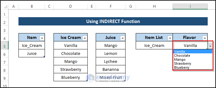
You will get the following drop-down option where you can select any flavor. Here, we get the following flavors for ice cream.

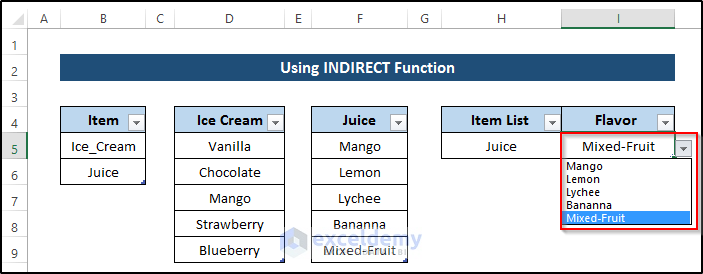
If we choose juice from the item list, the flavor will change accordingly.

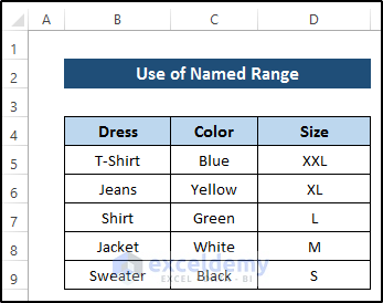
Method 2 – Use of Named Range

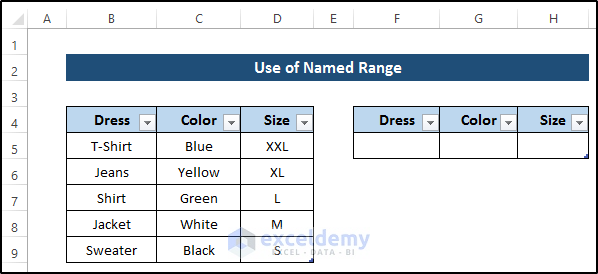
Let’s take a dataset that includes dress, color, and size.

Steps

Select the range of cells B4 to D9.

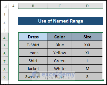
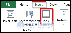
Go to the Insert tab on the ribbon.
Select Table from Tables group.

We will get a table.

Go to the Formulas tab on the ribbon.
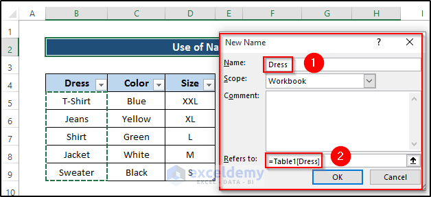
Select Define Name from the Define Names group.

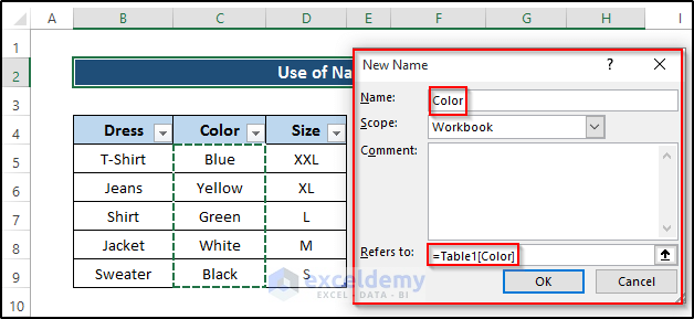
The New Name dialog box will appear. Set a name.
In the Refers to section, write down the following:

=Table1[Dress]

Click on OK.

Select Define Name from the Define Names group again.
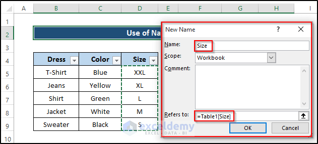
The New Name dialog box will appear. Set the next name.
In the Refers to section, write down the following:

=Table1[Color]

Click on OK.

Repeat for Size.

Create three new columns.

Select F5.
Go to the Data tab on the ribbon.
Select the Data validation drop-down option from the Data Tools group.

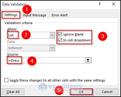
The Data Validation dialog box will appear.
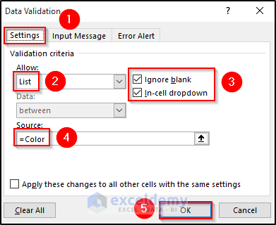
Select the Settings tab on the top.
Select List from the Allow.
Check the Ignore blank and In-cell dropdown options.
Write down the following in the Source section.

=Dress

Click on OK.

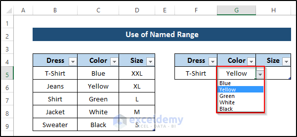
We will get the following drop-down options for the dress.

Select G5.
Go to the Data tab on the ribbon.
Select the Data validation drop-down option from the Data Tools group.

The Data Validation dialog box will appear.
Select the Settings tab on the top.
Select List in the Allow section.
Check the Ignore blank and In-cell dropdown options.
Write down the following in the Source section.

=Color

Click on OK.

We will get the following drop-down options for the color

Select H5.
Go to the Data tab on the ribbon.
Select the Data Validation drop-down option from the Data Tools group.

The Data Validation dialog box will appear.
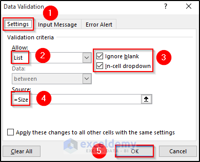
Select the Settings tab on the top.
Select List from the Allow section.
Check the Ignore blank and In-cell dropdown options.
Write down the following in the Source section.

=Size

Click on OK.

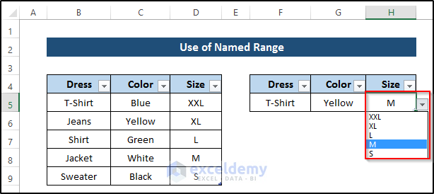
We will get the following drop-down options for the size.

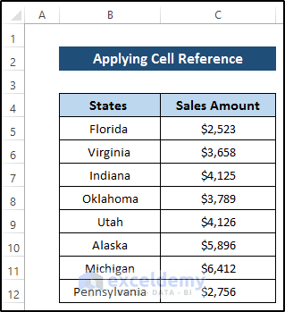
Method 3 – Applying Cell References in Data Validation

Let’s take a dataset that includes states and their sales amount.

Steps

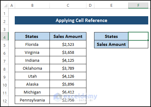
Create two new cells including states and sales amount.
Select cell F4.

Go to the Data tab on the ribbon.
Select the Data Validation drop-down option from the Data Tools group.

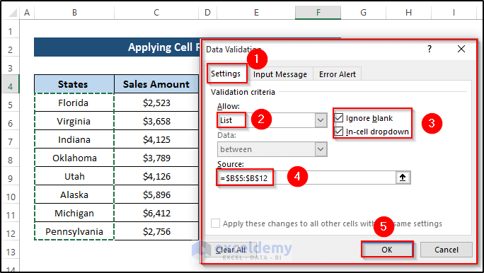
The Data Validation dialog box will appear.
Select the Settings tab on the top.
Select List from the Allow section.
Check the Ignore blank and In-cell dropdown options.
Select the range of cells B5 to B12.
Click on OK.

You will get a drop-down option where you can select any state.

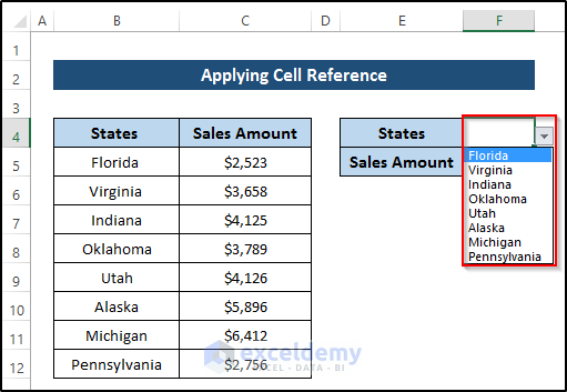
We would like to get the sales amount of the corresponding state. So, select cell F5.
Write down the following formula using the VLOOKUP function:

=VLOOKUP(F4,$B$5:$C$12,2,0)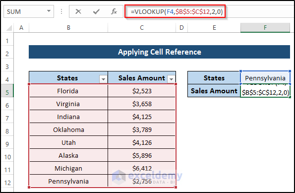

Click on Enter to apply the formula.

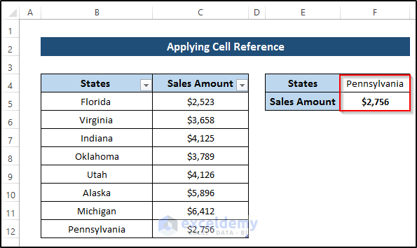
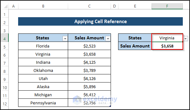
If you change the state from the drop-down option, the sales amount will change automatically.

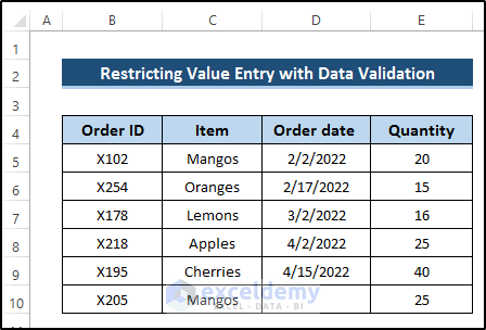
Method 4 – Restrict Value Entry with Data Validation

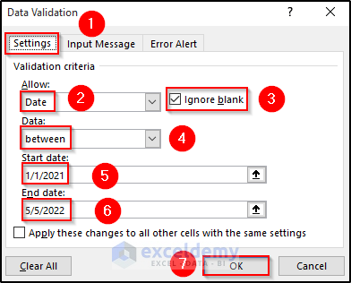
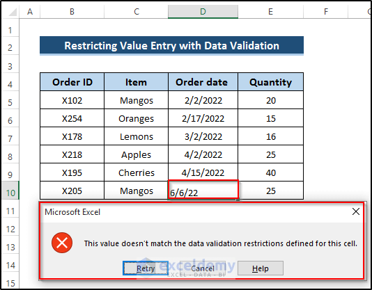
Consider a dataset that includes order ID, item, order date, and quantity. We would like to restrict the order date from 1 January 2021 to 5 May 2022.

Steps

Select cell D10.
Go to the Data tab on the ribbon.
Select the Data Validation drop-down option from the Data Tools group.

The Data Validation dialog box will appear.
Select the Settings tab on the top.
Select Date from the Allow section.
Check the Ignore blank option.
Select the between option from the Data section.
Set the start and end dates.
Click on OK.

If we put a date on cell D10 which is outside of the range, Excel will throw an error.

How to Do Data Validation Based on Adjacent Cell in Excel

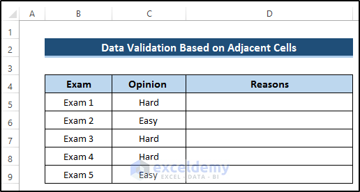
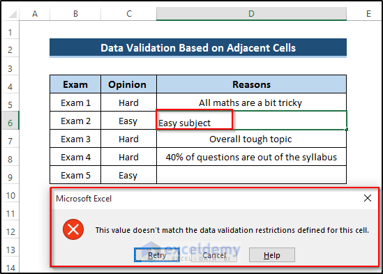
Let’s use a dataset that includes several exams, opinions, and reasons. We would like to be able write something in the reasons column only if the exam opinion is hard.

Steps

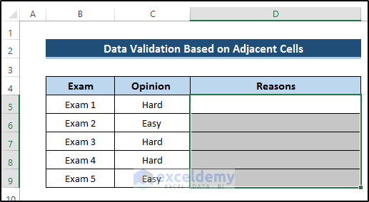
Select the range of cells D5 to D9.

Go to the Data tab on the ribbon.
Select the Data Validation drop-down option from the Data Tools group.

The Data Validation dialog box will appear.
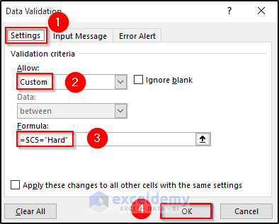
Select the Settings tab on the top.
Select Custom from the Allow section.
Write down the following formula in the Formula section.

=$C5="Hard"

Click on OK.

You can add descriptions in the reasons columns when the adjacent cell value is Hard.
If we try to add a description when the adjacent cell value is different, then it will show an error.

Download Practice Workbook

Download the practice workbook below.

Data Validation Based on Another Cell.xlsx

<< Go Back to Excel Custom Data Validation | Data Validation in Excel | Learn Excel

Get FREE Advanced Excel Exercises with Solutions!

19 Comments

Surya Jun 12, 2018 at 7:22 AM

Thank you for the article, it’s useful, short and well explained.
- Reply
  Siam Hasan Khan Jun 12, 2018 at 4:09 PM
  
  Thanks for your feedback, Surya.
NIlesh Oct 10, 2019 at 7:38 AM

Thanks this was helpful
- Reply
  Kawser Oct 10, 2019 at 12:59 PM
  
  Most welcome, Nilesh 🙂
Rodolfo Florano Oct 16, 2019 at 10:19 AM

Thanks a lot for sharing. Well explained
- Reply
  Kawser Oct 16, 2019 at 8:33 PM
  
  You’re welcome, Florano!
Jennifer Aug 27, 2021 at 7:23 PM

Why when I put in the formula =Items, excel gives me an error message and says that there is a problem with the formula? I formatted as tables and followed all the steps. Excel even recognizes the name and goes there, but gives the error message. Thanks
- Reply
  Thor Feb 23, 2022 at 2:19 PM
  
  It’s kind of old but maybe it will be useful for someone else in the future.
  When You use data validation u have to enter Named range in list range.
  If you enter table name You will get message about bad formula.
  I personaly dont like Named ranges because it’s troublesome to add new values.
  Instead I use only Tables. In Data Validation I use =INDIRECT(“TableName”) instead =TableName
  It works like a charm and Table keep it’s size by itself.
  - Reply
    Rafiul Haq Aug 8, 2022 at 4:41 PM
    
    Thank you for your reply, Thor.
Pipi Hema Mar 23, 2022 at 4:13 PM

Looking for help.. I have a spread sheet with data validations and formulas that once I select a piece of material from the list the cell populates with the price referenced on another sheet.

=IFERROR(VLOOKUP(B25,’Material Pricing’!$A$2:$C$313,3,0),””)

I want to be able to change the year on sheet 1 i.e from 2023 to 2024 (from a separate cell) and once I select the material from a dropdown have the price value change to reference the corresponding values in the column under that year which is in the other sheet.

Can this be done?
- Reply
  Rafiul Haq Aug 8, 2022 at 4:50 PM
  
  You can do this by combining IF function with your formula.
  Create multiple tables for your price information for the years. Refer the year to a cell and the use it to change the VLOOKUP’s “table_array”.
  
  For example the year is on cell F4,
  
  now you can type, =IF(F4=2023,IFERROR(VLOOKUP(B5,’Material Pricing’!B5:D7,3,0),””),IF(F4=2024,IFERROR(VLOOKUP(B5,’Material Pricing’!B13:D15,3,0),””),””))
  
  If the year is 2023, then the “table_array” will be B5:D7
  IF 2024, it will be B13:D15.
  Else it will return a blank.
  
  To know more about this, you can read this.
Anil Aug 5, 2022 at 8:29 PM

thanks, I was looking for this!!!
One question – do we need to have an Underscore “_” or dash “-” between two words in the Name range or Name cell?
- Reply
  Rafiul Haq Aug 8, 2022 at 4:37 PM
  
  Thank you for your question. You need to use Underscore (“_”) between two words in the Name Range.
Ash Aug 10, 2022 at 6:45 PM

Hi Guys,

I need some help in creating a data validation. I want to essentially be able to select the data from a list, which I am able to do, but then, basis that selection in the next cell I want items specifically from that list.

Eg. I apply a formula in Cell Z2 so that it lets me select from that list 🙂
in Cell AA2 now, I want to be able to reference that so that I only get the options that are relative to the value I selected in Z2. Is that possible?
- Reply
  Rafiul Haq Aug 11, 2022 at 5:06 PM
  
  Hey Ash, thank you for your question.
  
  Suppose, we have these three items in cell Z2 as a Dropdown List:
  X
  Y
  Z
  Then, if we choose X, then it should display as a list in AA2 cell:
  P
  Q
  R
  
  Now, to do that, select cell range that contains PQR (eg. T1:T3), then use Name Range
  PQR as X. Similarly, name the ranges as Y and Z for their corresponding cell ranges.
  
  Next, use Data Validation on cell AA2.
  Allow: List
  Source: =INDIRECT(Z2)
  
  Then, it should do what you want.
  
  TLDR; Use Name Range and INDIRECT function inside Data Validation.
Mary Aug 12, 2022 at 5:02 AM

Can you please explain why you use separate sheets instead of just one sheet for your tables? I have always used on sheet, labelled “LISTS” for all of my data validation tables. The reason I’m here now is because I need to select data from one list based on data in another list. I’m not sure why this would need more than one sheet.
Thanks.
- Reply
  Nahian Aug 17, 2022 at 11:44 AM
  
  Hi Mary, thanks for your response. You can definitely apply this process in a single sheet. However we use different sheets to show the different processes for the same output. And it also seemed convenient to use separate sheets to show the application of using the data validation list for different conditions. So different sheets for different methods were used in this article. Hope that provides you with the answer to your question.
Steve V Aug 17, 2022 at 7:33 PM

incredibly confusing. there is no need to format as table. Just create the filter in the header row. using named ranges prevents people from intuitively understanding what range you’re talking about – REFERENCE RANGES EXPLICITLY! tutorials should not use either named ranges or references to other sheets. that just makes it more difficult to understand. set up your example on one sheet and let US move lookup tables to other sheets as needed.
- Reply
  Nahian Aug 22, 2022 at 11:10 AM
  
  Hi Steve, we are extremely sorry for your trouble. Named ranges are pretty useful when we need to use a range repeatedly. A lot of our readers are okay with it. Going through the dataset can help anyone to understand the defined range of a named range. But we are taking your feedback sincerely. We’ll apply your suggestion in the upcoming articles.

Data Validation Based on Another Cell in Excel (4 Examples)

How to Do Data Validation in Excel?

Method 1 – Applying INDIRECT Function

Method 2 – Use of Named Range

Method 3 – Applying Cell References in Data Validation

Method 4 – Restrict Value Entry with Data Validation

How to Do Data Validation Based on Adjacent Cell in Excel

Related Articles

Leave a reply Cancel reply