In the following GIF, we display the unit price of the selected products in 2 different stores: Walmart and Kroger. We applied the VLOOKUP function with the IF condition to extract the unit prices. The Data Validation drop-down list is being used to select the store and product.
What Is the Excel IF Function?
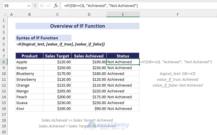
The IF function in Excel tests a condition. If the condition is met, it returns one specified value. Otherwise, it returns another specified value.
The following overview image shows how the function is used to determine the status of different products based on the sales target and sales achieved.
What Is the Excel VLOOKUP Function?
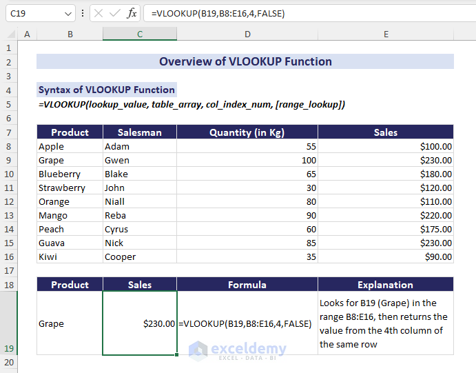
The VLOOKUP function looks for a specified value in the leftmost column of a given table and returns the value in the same row from the specified column relative to the start of the lookup table.
The following overview image shows the use of the function to extract the sales of Grape from the table.
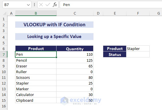
Example 1 – Looking Up a Specific Value by Combining VLOOKUP with IF
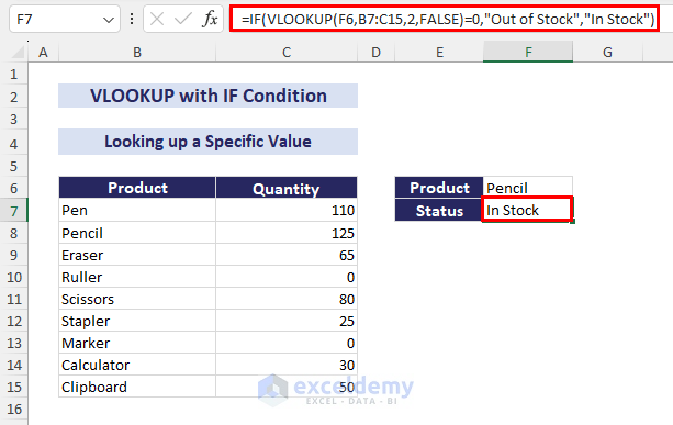
We have some products and their respective quantities. We’ll check whether a selected product is in stock based on the quantity and then display its status.
Steps:
- Select cell F7.
- Insert the following formula into the cell:
=IF(VLOOKUP(F6,B7:C15,2,FALSE)=0,"Out of Stock","In Stock")- Press Enter.
Formula Breakdown
=IF(VLOOKUP(F6,B7:C15,2,FALSE)=0,”Out of Stock”,”In Stock”)
=IF(125=0,”Out of Stock”,”In Stock”) // VLOOKUP(F6,B7:C15,2,FALSE) returns 125 because F6 (Pencil) is found in the 2nd row of the range B7:C15 and the intersection of 2nd row and 2nd column is 125.
=In Stock // IF(125=0,”Out of Stock”,”In Stock”) returns “In Stock” as 125 is not equal to 0 in the logical test.
The following GIF displays the status of a few products randomly. We selected the products using the Data Validation drop-down list.
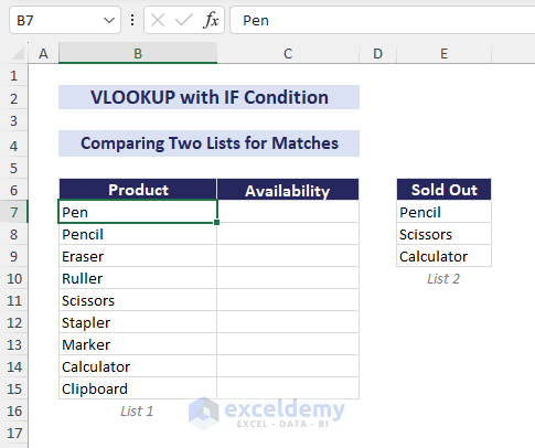
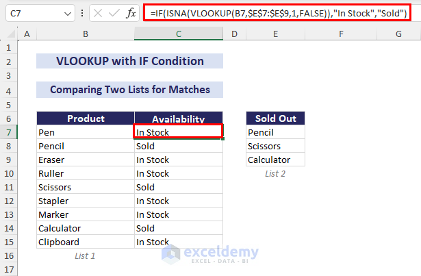
Example 2 – Comparing Two Lists for Matches Using VLOOKUP, IF, and ISNA Functions in Excel
We have 2 lists where List 1 has some products and List 2 has only the sold-out products. We’ll check the availability of products in List 1 by checking if they (don’t) exist in List 2.
Steps:
- Select the cell C7.
- Insert the following formula:
=IF(ISNA(VLOOKUP(B7,$E$7:$E$9,1,FALSE)),"In Stock","Sold")- Press Enter and drag the Fill Handle down to fill the column.
Read More: How to Use IF ISNA Function with VLOOKUP in Excel
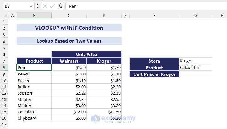
Example 3 – Using VLOOKUP and IF to Lookup Based on Two Values
We have some products and their unit prices in 2 different stores: Walmart and Kroger. We’ll extract the unit price of a selected product from the specified store.
Steps:
- Select cell G9.
- Insert the following formula:
=IF(G7="Walmart",VLOOKUP(G8,B8:D16,2,FALSE),VLOOKUP(G8,B8:D16,3,FALSE))- Press Enter.
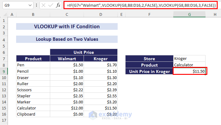
- The following GIF shows the unit price of the products. We select the product and the store using Data Validation drop-down lists.
You can also use the following formula:
=VLOOKUP(G8,B8:D16,IF(G7="Walmart", 2, 3),FALSE)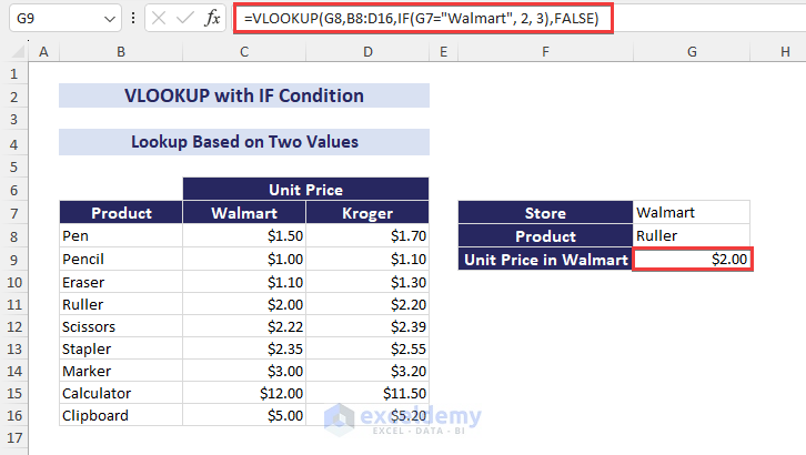
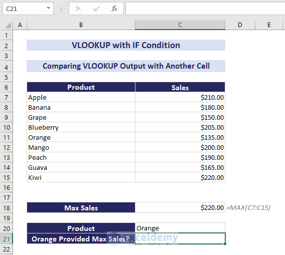
Example 4 – Comparing the VLOOKUP Output with Another Cell Value in Excel
The dataset contains some products and their corresponding sales. We’ll fetch the maximum sales by using the MAX function formula:
=MAX(C7:C15)We’ll determine which product has generated the maximum sales by comparing the sales figures with the MAX formula’s output.
Steps:
- Select cell C21.
- Insert the formula:
=IF(VLOOKUP(C20,B7:C15,2,FALSE)>=C18,"Yes","No")- Press Enter.
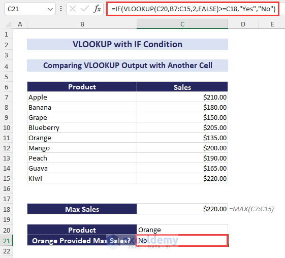
- The following GIF compares the sales figures of the selected products with the maximum sales value. In this example, we selected the product using the Data Validation drop-down list.
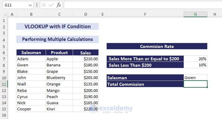
Example 5 – Performing Multiple Calculations by Using VLOOKUP with IF Condition
We have a dataset of salespeople with their respective product and sales. We’ll determine the total commission of a salesperson based on their sales. For those who have sales greater than or equal to $200, the commission rate is 20%. Otherwise, they will receive a 10% commission.
Steps:
- Select cell G11.
- Insert the following formula:
=IF(VLOOKUP(G10,B7:D15,3,FALSE )>=200, VLOOKUP(G10,B7:D15,3,FALSE)*G7, VLOOKUP(G10,B7:D15,3,FALSE)*G8)- Press Enter.
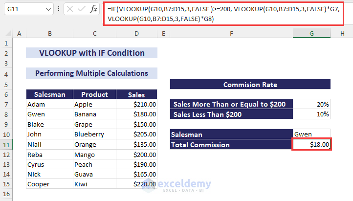
- The following GIF finds out the total commission of the selected salesperson. We select the name using a Data Validation drop-down list.
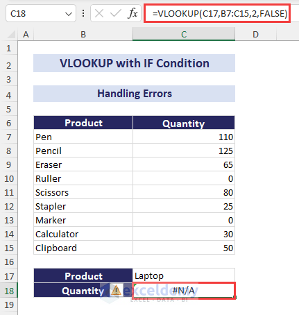
Example 6 – Handling Errors in VLOOKUP with IF Condition in Excel
In the following image, the Laptop is not found in the product list of the dataset and the formula returns the #N/A error. We’ll remove this error value.
- To display a particular text e.g. Not Found, when the lookup value is not found, use the following formula:
=IF(ISNA(VLOOKUP(C17,B7:C15,2,FALSE)), "Not Found", VLOOKUP(C17,B7:C15,2,FALSE))- For displaying 0 when the lookup value is not found, use the formula:
=IF(ISNA(VLOOKUP(C17,B7:C15,2,FALSE)), 0, VLOOKUP(C17,B7:C15,2,FALSE))- To display a blank cell when the lookup value is not found, use the formula:
=IF(ISNA(VLOOKUP(C17,B7:C15,2,FALSE)), "", VLOOKUP(C17,B7:C15,2,FALSE))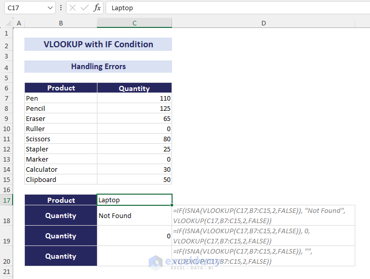
NOTE: ISNA is available in all Excel versions. But we have to use ISNA with IF to deal with the error. On the other hand, IFNA can handle #N/A errors without using IF. IFNA is available in Excel 2013 and later versions.
To handle all sorts of errors (not only #N/A) combine VLOOKUP with the IFERROR function.
Download the Practice Workbook
VLOOKUP with IF: Knowledge Hub
<< Go Back to Excel VLOOKUP Function | Excel Functions | Learn Excel
Get FREE Advanced Excel Exercises with Solutions!

In the 4th way, I commonly use MATCH instead IF, because if I have more than two items, MATCH works very well
The col_index argument will be like this:
MATCH($C$14,$B$4:$E$4,0)
By the way, great job!! Keep going!
Have a nice day!
Hi Daniel,
Thanks for your feedback.
Yes. INDEX and MATCH combo work in a more versatile way than the VLOOKUP function. I did not use Index Match because I wanted to show all the examples with VLOOKUP and IF Functions.
Keep in touch.
Best regards
Kawser
interesting function & I can’t dispense it <3
Thanks for your feedback 🙂
Congratulations, great!
I want to user function which you shown in screen in VBA code , but it’s not run.
I m using 3 different sheet.
1 sheet lookup value pick d2 col and also check f2 value .
Range another sheet2 case 1 and case 2,value need
And results sheet3
Thanks, Ferreira!
Thank you for the useful tutorial, it explained the uses very easily and effectively. 🙂
Nice code, but your explanations are rather condescending. “For the complete layman”…? Comes off as superior.
Maybe a little bit tough for the complete layman. I shall change my Phrase then 🙂
Hi,
I’m struggling to find the right formula to multiply units by rates.
I have different materials and tasks with different units and rates are depend on quantities. Some of the units only have one rate with no conditions.
I have a more than 2000 row spreadsheet and units also varies that means that the formula also need to find the unit on sheet 1. Rate criteria can also change on sheet 1.
I’m looking for the price on Sheet2.
I believe the below formula need to be combined with vlookup but I cannot get it to work
‘=IF(C210,C250,C2200,C2*G2,0))))
Many thanks for your help!
Niki
Sheet 1
Unit”Rate1(not exceeding)””Rate2(not exceeding)””Rate3(not exceeding)””Rate4(exceeding)”
day
h
m (QB) 10 50 200 200
m
m2 (QB) 10 50 150 150
m2
Sheet 2
Description Unit Quantity Rate 1 Rate 2 Rate 3 Rate 4 Price
path m (QB) 10 11 13 13.5 14
road m (QB) 51 5 10 15 20
wall m2 (QB) 35 10 15 20 25
wood m 20 11
paint m2 150 12
Is there a way to add another criteria to this formula? I want to add if this range has a certain word, in my case OUTSTANDING, to return BLANK””. Current Formula: IFERROR(VLOOKUP(B9,’REPORT!A:C,3,FALSE),””)
Hi there!
I couldn’t fully understand what you need from your comment. However, I assumed you may want to create something like the following formula.
=IFERROR(IF(REPORT!A:C="OUTSTANDING","",VLOOKUP(B9,REPORT!A:C,3,FALSE)),"")Is this what you needed? If not, then tell us more about the problem so that we may help you. Thank you for being with us.
Regards
Md. Shamim Reza (ExcelDemy Team)
I am trying to get a value from a table that matches text from a list. I feel like this should do it, but i get an error code each time.
=IF(VLOOKUP(F52,C17:G24,5,FALSE))
What am I missing here?
Hello Ty Calkins,
The issue with your formula lies in the use of the IF function. In Excel, IF requires three arguments: a condition, a result if the condition is true, and a result if the condition is false. You’re missing those components in your current formula.
Correct Formula:
=IF(ISERROR(VLOOKUP(F52,C17:G24,5,FALSE)), “Value not found”, VLOOKUP(F52,C17:G24,5,FALSE))
VLOOKUP(F52, C17:G24, 5, FALSE): This looks for the value in F52 within the range C17:G24 and returns the value from the 5th column.
ISERROR: This checks if the VLOOKUP produces an error (e.g., if the value is not found).
“Value not found”: This is the result if the VLOOKUP results in an error.
VLOOKUP(F52, C17:G24, 5, FALSE): This is the result if the VLOOKUP successfully finds a match.
Regards
ExcelDemy