Practical Uses
1. How to Match VLOOKUP Output with a Specific Value
Let’s say we want to determine how much inventory we have for a particular product.
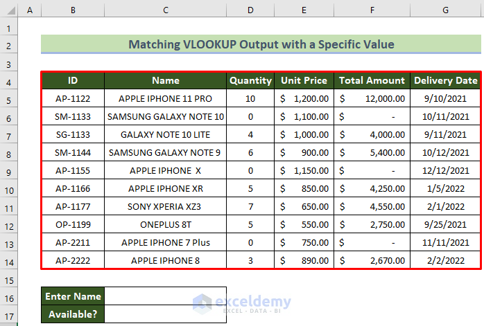
Steps:
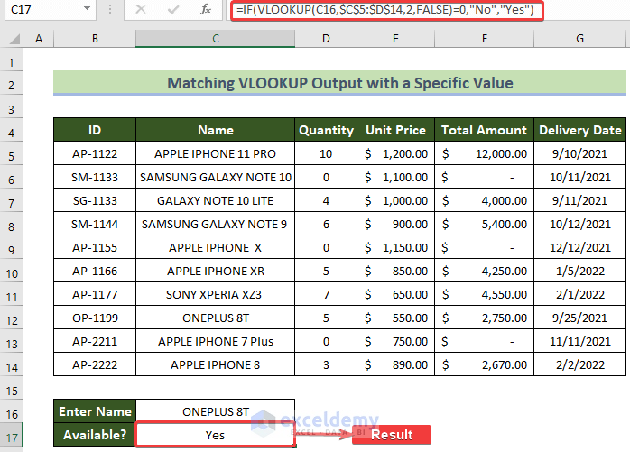
- Select C17 and enter the following formula:
=IF(VLOOKUP(C16,$C$5:$D$14,2,FALSE)=0,"No","Yes")- Press Enter.
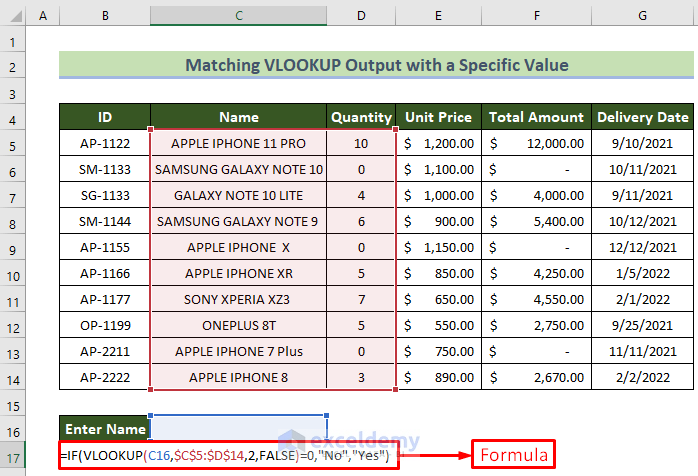
Formula Breakdown:
- VLOOKUP in C16 identifies Name as the search keyword.
- $C$5:$D$14 identifies the search range; the 2 means we are looking for matching criteria in the second column (Quantity), while FALSE means we have an exact match.
- The formula VLOOKUP(C16,$C$5:$D$14,2, FALSE) calculates the Quantity of product assigned to that
- With the addition of the IF function, i.e. depending on whether the result is greater than zero, C17 indicates either Yes (the product is in stock) or No (the product is not currently in stock).
Note that if the product in C16 indicates a quantity greater than zero in D16, the result appears as Yes.
Note that if the product in C16 indicates a quantity equal to zero in D16, the result appears as No.
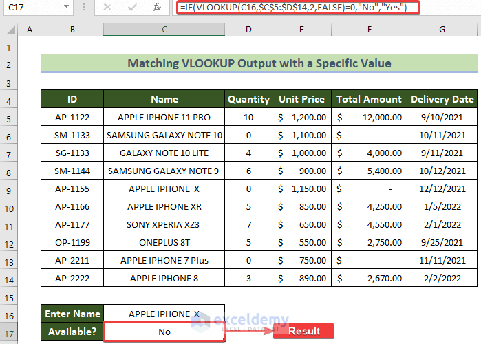
We now know that the Apple iPhone X is not in stock.
Read More: How to Use Nested VLOOKUP in Excel
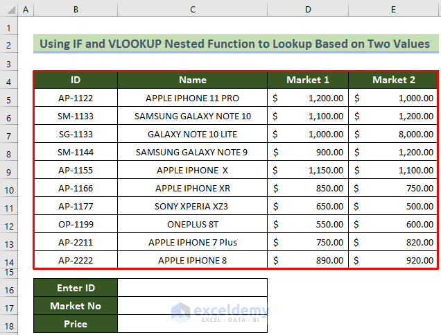
2. How to Use the IF & VLOOKUP Nested Function With Two Lookup Values
Let’s say we want to locate the price of a particular product in a particular market.
Steps:
- Select C18 and enter the following formula:
=IF(C17="Market 1",VLOOKUP(C16,B5:E14,3,FALSE),VLOOKUP(C16,B5:E14,4,FALSE))- Press Enter.

- Select C16 and enter the product’s ID.
- Select C17 and enter Market 1.
- Press Enter.
Formula Breakdown:
- IF(C17=”Market 1″) determines that our initial interest is in Apple iPhone X’s Market 1 price.
- VLOOKUP(C16,B5:E14,3,FALSE) identifies the search range, i.e. the third column (Market 1).
- IF(C17=”Market 1″,VLOOKUP(C16,B5:E14,4,FALSE) means that if there is no Market 1 price, the search moves on to the fourth column (Market 2).
- When the Apple iPhone X’s ID is entered in C16 and “Market 1” in C17, the price will appear in C18.
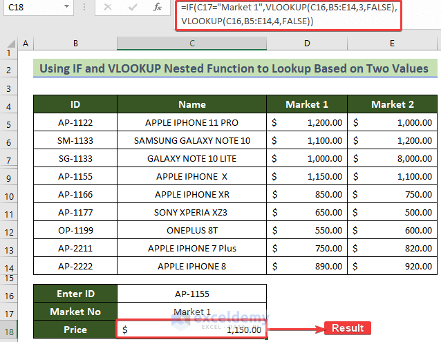
We now know that the Market 1 price for the Apple iPhone X is $1,150.00.
Read More: Excel LOOKUP vs VLOOKUP
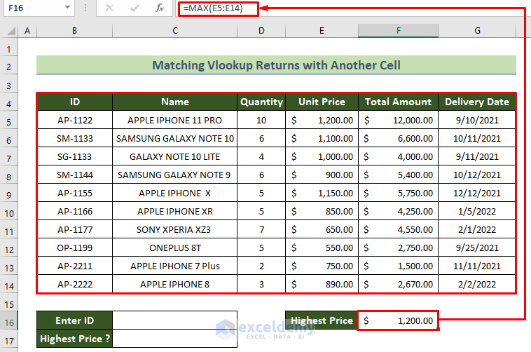
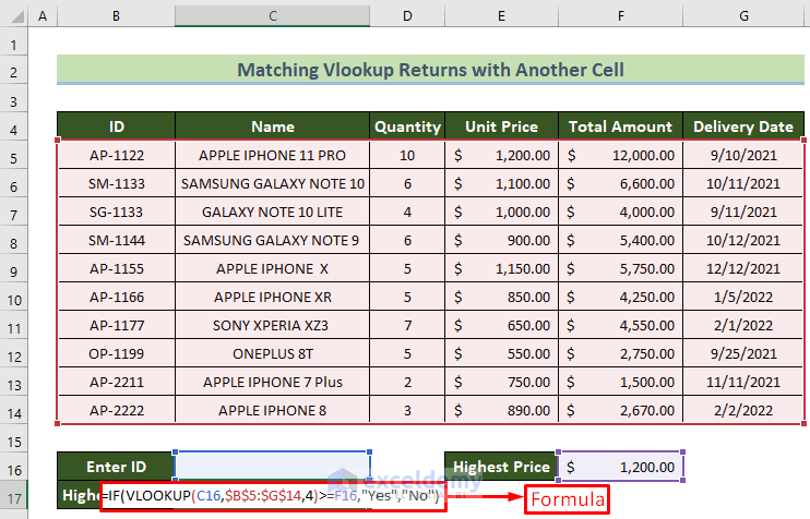
3. How to Match Lookup Returns with Another Cell Using the MAX Function
Let’s say we want to compare unit prices across products to see which is the highest.
Steps:
- Select C17 and enter the following formula:
=IF(VLOOKUP(C16,$B$5:$G$14,4)>=F16,"Yes","No")- Press Enter.
Formula Breakdown:
- VLOOKUP(C16,$B$5:$G$14,4) compares the Apple iPhone 11 Pro’s Unit Price with that of the highest price (calculated in Example 3).
- IF >=F16,”Yes”,”No” determines whether that price is greater than or equal to the price in F16.
- IF(VLOOKUP(C16,$B$5:$G$14,4) >=F16,”Yes”,”No” compares these prices, then indicates Yes or No in C17.
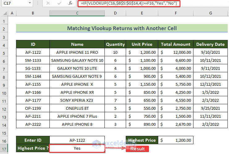
We now know that the most expensive product we sell is the Apple iPhone 11 Pro.
Read More: Return the Highest Value Using VLOOKUP Function in Excel
4. How to Use the IF & VLOOKUP Nested Function to Lookup Values from a Shorter List
Let’s say we want to find out whether a particular product has been delivered.
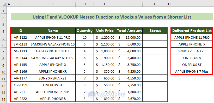
Steps:
- Select G5 and enter the following formula:
=IF(ISNA(VLOOKUP(C5,$I$5:$I$10,1,FALSE)),"Not Delivered","Delivered")- Press Enter.
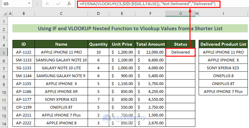
Formula Breakdown:
- IF establishes the delivery status of each product as Delivered or Not delivered
- ISNA sets the criterion as TRUE (if delivered) or FALSE (if not).
- VLOOKUP(C5,$I$5:$I$10,1, FALSE) checks the Name of each product and, if it matches TRUE, adds it to the Delivered Project List (column I), then indicates Delivered or Not delivered in G5.
To duplicate the formula, click and drag the Fill Handle down the targeted range.
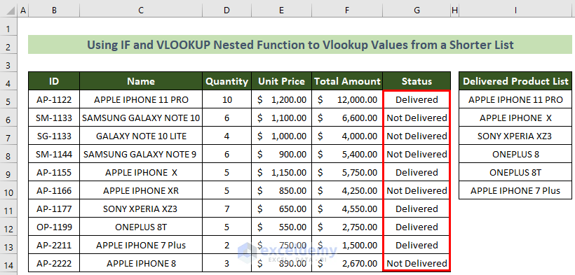
We now know that six of the ten products have been delivered.
5. How to Use the IF & VLOOKUP Nested Function to Perform Different Calculations
Let’s say we want to find out whether a) with a discount of 20%, the unit price is greater than $800 or b) with a discount of 15%, it’s lower than $800.
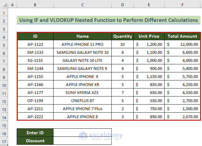
Steps:
- Select C17 and enter the following formula:
=IF(VLOOKUP(C16,$B$5:$F$14,4,FALSE )>800, VLOOKUP(C16,$B$5:$F$14,4,FALSE)*15%, VLOOKUP(C16,$B$5:$F$14,4,FALSE)*20%)- Press Enter.
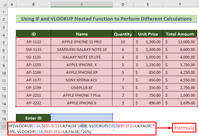
Formula Breakdown:
- IF establishes that the Unit Price is either over or under 800.
- VLOOKUP(C16,$B$5:$F$14,4,FALSE )>800 checks whether the product ID entered in C16 has a Unit Price greater than 800.
- =IF(VLOOKUP(C16,$B$5:$F$14,4,FALSE )>800,VLOOKUP(C16,$B$5:$F$14,4,FALSE)*15%,VLOOKUP(C16,$B$5:$F$14,4,FALSE)*20%) ensures that the product’s unit price is correctly multiplied by 15% (if greater than 800) or 20% (if less than 20%), ), then indicates the Discount in C17.
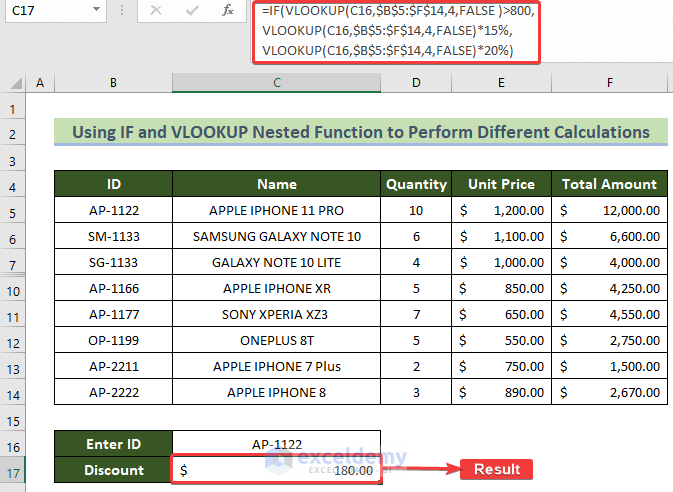
We now know the discounted price for the Apple iPhone 11 Pro is $180 less than its unit price.
Handling Errors
Sometimes there’s no match to your lookup, so you might get #N/A or 0.

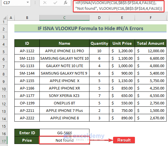
1. How to Use the ISNA Function with the IF & VLOOKUP Nested Function to Hide #N/A Errors
Steps:
- Select C17 and enter the following formula:
=IF(ISNA(VLOOKUP(C16,$B$5:$F$14,4,FALSE)),"Not found",VLOOKUP(C16,$B$5:$F$14,4,FALSE))- Press Enter.
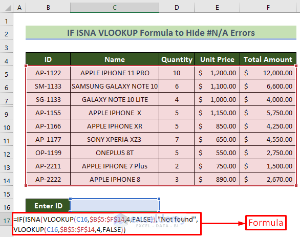
Formula Breakdown:
- IF establishes that each product in the dataset may or may not have a unit price.
- VLOOKUP(C16,$B$5:$F$14,4,FALSE) searches Unit Price (column E) for the product ID entered in C16.
- ISNA(VLOOKUP(C16,$B$5:$F$14,4,FALSE)) checks whether or not the product has a unit price.
- =IF(ISNA(VLOOKUP(C16,$B$5:$F$14,4,FALSE)),”Not found”,VLOOKUP(C16,$B$5:$F$14,4,FALSE)) ensures C17 will indicate either the unit price (if the product has one) or “Not found” (if it doesn’t).
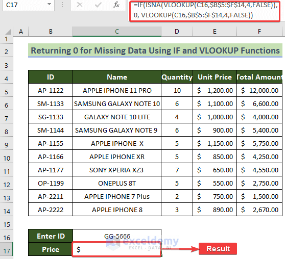
2. How to Use the ISNA Function with the IF & VLOOKUP Nested Function to Represent Missing Data as 0
Steps:
- Select C17 and enter the following formula:
=IF(ISNA(VLOOKUP(C16,$B$5:$F$14,4,FALSE)),0,VLOOKUP(C16,$B$5:$F$14,4,FALSE))- Press Enter.
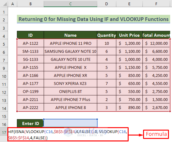
Formula Breakdown:
- IF establishes that each product may or may not have a unit price.
- ISNA(VLOOKUP(C16,$B$5:$F$14,4,FALSE)) searches Unit Price (column E) for the product ID entered in C16.
- =IF(ISNA(VLOOKUP(C16,$B$5:$F$14,4,FALSE)),0,VLOOKUP(C16,$B$5:$F$14,4,FALSE)) ensures C17 indicates either the unit price (if the product has one) or 0 (if it doesn’t).
Things to Remember
#N/A errors typically appear because:
- The lookup value does not exist in the table.
- The lookup value is misspelled or contains extra space.
- The table range was not entered correctly.
- You are copying VLOOKUP across several sells without first locking the table reference.
When cells are formatted as currently, there will be a dashed line (-) instead of 0.
Download Free Practice Workbook
Further Readings
- Combining SUMPRODUCT and VLOOKUP Functions in Excel
- How to Use VLOOKUP with COUNTIF
- How to Combine SUMIF and VLOOKUP in Excel
- Use VLOOKUP to Sum Multiple Rows in Excel
- INDEX MATCH vs VLOOKUP Function
- XLOOKUP vs VLOOKUP in Excel
- How to VLOOKUP and SUM Across Multiple Sheets in Excel
- How to Use IFERROR with VLOOKUP in Excel
<< Go Back to VLOOKUP with IF Condition | Excel VLOOKUP Function | Excel Functions | Learn Excel
Get FREE Advanced Excel Exercises with Solutions!

I need help.
I have two criteria data points to reference, to pull a third.
If A and B match on sheet 1 & 2, I need to pull in the third column’s data. How do I accomplish this? I believe I am overthinking this formula nesting.
Hello APRIL, We already have an article written based on your problem. I hope, you will find this helpful. Follow this link below-
https://www.exceldemy.com/excel-vlookup-multiple-criteria-without-helper-column/
Try the methods mentioned in this article and let us know the outcome. Thank you!