Understanding the Scenario
Let’s start with a basic example. Imagine we have a table with product names and their revenues over five months. We want to find the total revenue for a specific product using criteria (such as the product name).
Example 1 – Calculating Total Revenue
- Enter the following formula in cell E14:
=SUMPRODUCT(VLOOKUP(E13,B5:G11,{2,3,4,5,6},0))- Press Enter to get the result, which should be $940,000.
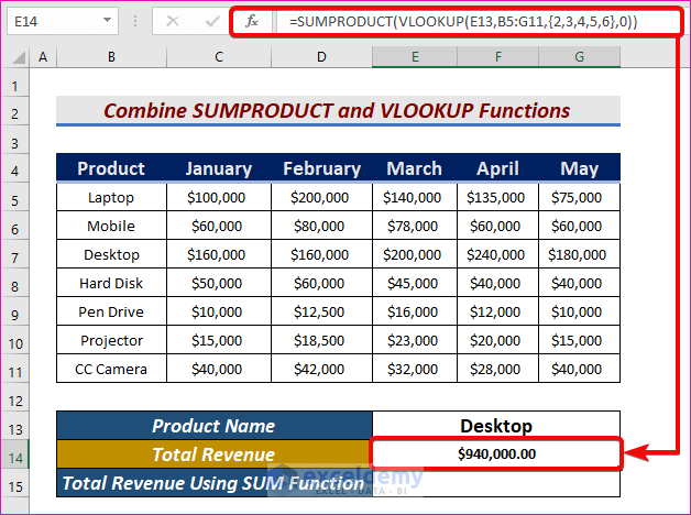
- Inside the VLOOKUP function:
- E13 is the lookup_value.
- B5:G11 is the lookup_array.
- {2,3,4,5,6} specifies the columns (C to G) from which we want values.
- 0 ensures an exact match.
- The SUMPRODUCT function multiplies the elements of the array returned by VLOOKUP and sums them up.
Using the SUM Function Instead
You can achieve the same result using the SUM function:
=SUM(VLOOKUP(E13,B5:G11,{2,3,4,5,6},0))
Note
- If the lookup array (B5:G11) doesn’t contain the lookup value, you’ll see #N/A.
- Using SUMPRODUCT with text in reference range cells may result in a #VALUE! error.
In the above discussion, we used the SUMPRODUCT and VLOOKUP functions to calculate the total revenue of a specific product. We can calculate the total revenue of a specific product using the SUM function instead of SUMPRODUCT. The formula will be:
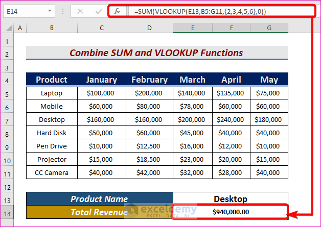
- Inside the VLOOKUP function:
- E13 is the lookup_value.
- B5:G11 is the lookup_array.
- 2 to 6 within curly braces is in the column_num field.
- 0 is used for the exact match.
- Finally, the SUM function calculates the total revenue earned from the product named Desktop.
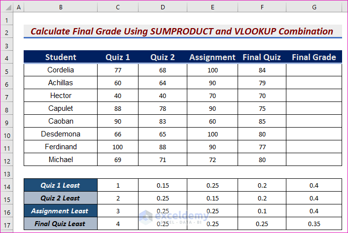
Example 2 – Calculate Final Grade Using SUMPRODUCT and VLOOKUP
In this section, we’ll determine the final grades for several students by combining the SUMPRODUCT and VLOOKUP functions. Our calculation criteria vary based on the student’s score.
Specifically:
- If a student scored lowest in Quiz 1, the weight will be 0.15, 0.25, 0.2, and 0.4 for Quiz 1, Quiz 2, Assignment, and Final Quiz, respectively.
Here are the steps:
- Multiply each score by its corresponding weight.
- Sum the weighted scores to obtain the final grade.
The formula for this is:
=SUMPRODUCT(C5:F5,VLOOKUP(MATCH(MIN(C5:F5),C5:F5,0),$C$14:$G$17,{2,3,4,5},0))- Press Enter to calculate. The result should be 83.05.
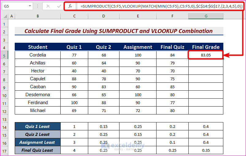
- We use the first array (C5:F5) for student scores.
- The second array is obtained using VLOOKUP, which finds the weight value corresponding to the lowest score. We use MATCH and MIN to determine the column number for the lowest value.
- Press F9 to see the insights (the MATCH portion will change based on the minimum value).
- The lookup_value for VLOOKUP is the result of MATCH(MIN(C5:F5), C5:F5, 0).
- The weighted table range ($C$14:$G$17) serves as the lookup_array, and 0 ensures an exact match.
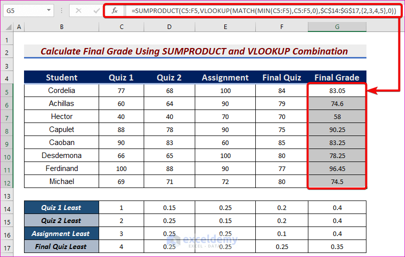
To calculate other students’ grades, follow the same process or use the AutoFill feature.
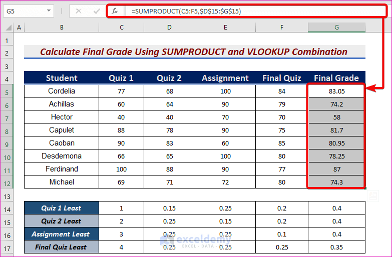
Additionally, you can directly verify the result using the SUMPRODUCT function:
- To clarify the result, use the SUMPRODUCT function directly. The SUMPRODUCT function is,
=SUMPRODUCT(C5:F5,$D$15:$G$15)- Where C5:F5 represents array1 (scores) and $D$15:$G$15 represents array2 (weights). You should obtain the same value as the SUMPRODUCT-VLOOKUP approach.
Read More: 7 Practical Examples of VLOOKUP Function in Excel
Download Practice Workbook
You can download the practice workbook from here:
Further Readings
- How to Use VLOOKUP with COUNTIF
- How to Combine SUMIF and VLOOKUP in Excel
- Use VLOOKUP to Sum Multiple Rows in Excel
- INDEX MATCH vs VLOOKUP Function
- Excel LOOKUP vs VLOOKUP
- XLOOKUP vs VLOOKUP in Excel
- How to Use Nested VLOOKUP in Excel
- IF and VLOOKUP Nested Function in Excel
- How to Use IF ISNA Function with VLOOKUP in Excel
- How to VLOOKUP and SUM Across Multiple Sheets in Excel
- How to Use IFERROR with VLOOKUP in Excel
- VLOOKUP with IF Condition in Excel
<< Go Back to Excel VLOOKUP Sum | Excel VLOOKUP Function | Excel Functions | Learn Excel
Get FREE Advanced Excel Exercises with Solutions!
