The sample sheets are for 3 consecutive months: January, February, and March, containing the Product Name, Product ID, and Sales for each month. We will see how to apply the VLOOKUP function for a value and get the result as the sum of the sales for 3 months.

Method 1 – Use VLOOKUP and SUM Functions Across Multiple Sheets
Steps:
- Select cell C5 and insert the following formula.
=SUM(VLOOKUP(B5,January!$B$5:$D$9,{3},FALSE),VLOOKUP(B5,February!$B$5:$D$9,{3},FALSE),VLOOKUP(B5,March!$B$5:$D$9,{3},FALSE))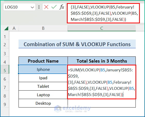
Formula Description:
- In the VLOOKUP function, we are looking up for Product Name in cell B5.
- We have added all the 3 sheets’ table ranges.
- The column index for the dataset for all the 3 sheets is 3 as we want the result of sales, which is in the D column, which is third in the range.
- We wanted an exact match, so we put FALSE. You can use TRUE in case you want an approximate match.
- The SUM function provides the sum of the matched items.
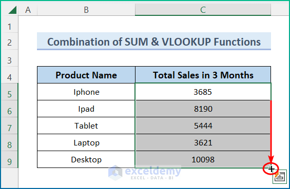
- Hit the Enter button and utilize the AutoFill tool to the entire column.
Read More: How to Use VLOOKUP Function with Exact Match in Excel
Method 2 – VLOOKUP and Sum Across Multiple Sheets Applying SUMPRODUCT, SUMIF, and INDIRECT Functions
Steps:
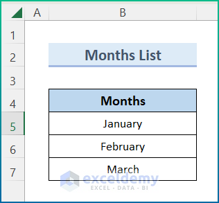
- Write the sheet names and select them.
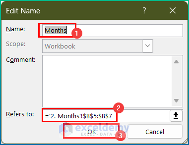
- Click on the Define Name from the Formulas tab.
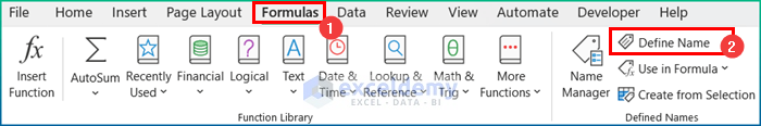
- Write “Months” in the Name section.
- Check the range in Refers to: and click OK.
- Insert the formula below in cell C5 to get results for sales of 3 months for Product ID #1101.
=SUMPRODUCT(SUMIF(INDIRECT("'"&Months&"'!C5:C9"),$B$5,INDIRECT("'"&Months&"'!D5:D9")))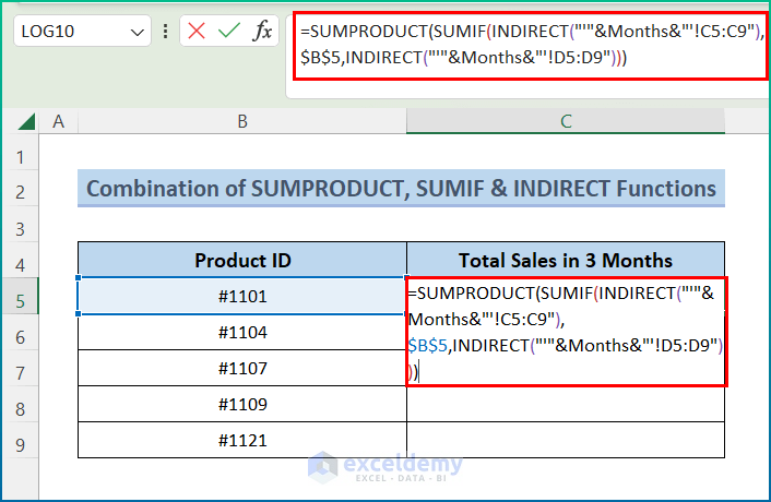
Formula Description:
- The INDIRECT function returns the reference specified by a text string. For this dataset, we have used the “Months” list which we created at the beginning of the process.
- The SUMIF function checks the range and criteria to find the desired sum.
- The SUMPRODUCT function takes arrays and gives the sum of the products of the corresponding ranges and arrays received already.
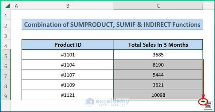
- Press Enter and apply the AutoFill tool to the whole column in order to get your desired output.
Read More: VLOOKUP with IF Condition in Excel
Things to Remember
- You must follow the syntax of the formulas if you have a different dataset.
- To write arguments from different sheets, you can simply click on the sheet and select the required data.
- Formulas will get longer with the number of sheets you have in your dataset for the first method, but the second method solves that nicely.
Download the Practice Workbook
Related Readings
- Combining SUMPRODUCT and VLOOKUP Functions in Excel
- How to Use VLOOKUP with COUNTIF
- How to Combine SUMIF and VLOOKUP in Excel
- Use VLOOKUP to Sum Multiple Rows in Excel
- INDEX MATCH vs VLOOKUP Function
- Excel LOOKUP vs VLOOKUP
- XLOOKUP vs VLOOKUP in Excel
- How to Use Nested VLOOKUP in Excel
- IF and VLOOKUP Nested Function in Excel
- How to Use IF ISNA Function with VLOOKUP in Excel
- How to Use IFERROR with VLOOKUP in Excel
<< Go Back to VLOOKUP Between Worksheets | Excel VLOOKUP Function | Excel Functions | Learn Excel
Get FREE Advanced Excel Exercises with Solutions!
