How to Use VLOOKUP Formula in Excel with Multiple Sheets

An Introduction to Excel’s VLOOKUP Function

=VLOOKUP(lookup_value,table_array,col_index_num,[range_lookup])

This function takes a range of cells called table_array as an argument.
Searches for a specific value called lookup_value in the first column of the table_array.
Looks for an approximate match if the [range_lookup] argument is TRUE, otherwise searches for an exact match. Here, the default is TRUE.
If it finds any match of the lookup_value in the first column of the table_array, it moves a few steps right to a specific column (col_index_number), and returns the value from that cell.

The image below shows an example of this VLOOKUP function.

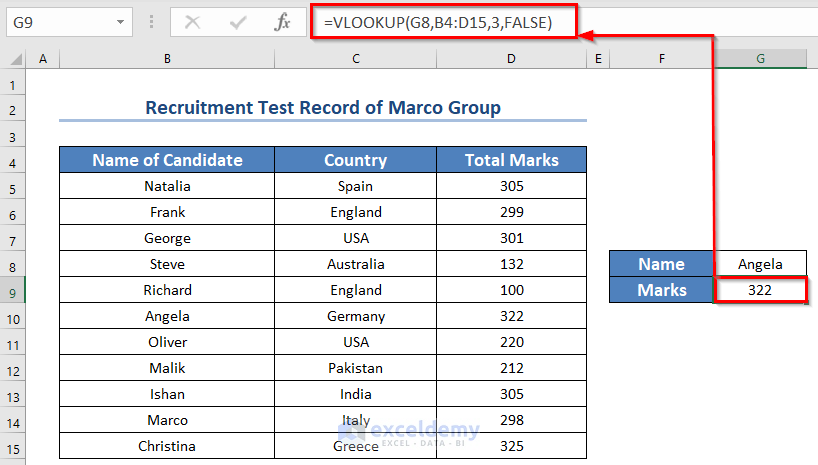
Formula Breakdown

The formula VLOOKUP(G8,B4:D15,3,FALSE) searched for the value of G8 cell “Angela” in the first column of the table: B4:D15.

After it found one, it moved right to the 3rd column (As the col_index_number is 3).

The value from there was 322.

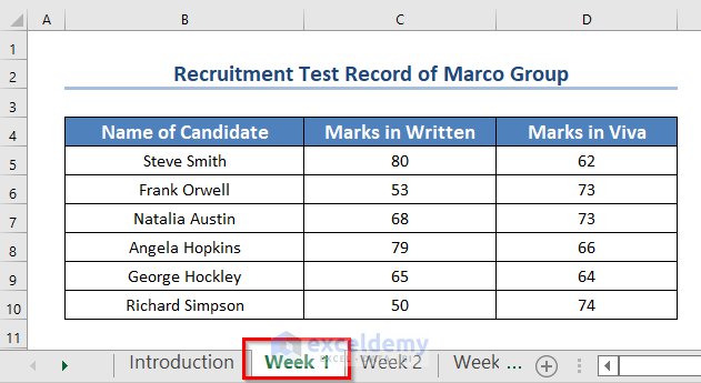
This sample workbook shows the written and viva exam scores of several candidates. The scores are divided into three separate worksheets, each representing a different week. The first worksheet is labeled Week 1.

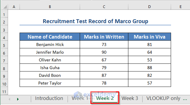
The 2nd worksheet is Week 2.

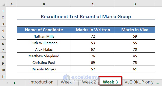
The 3rd worksheet is Week 3.

Our objective is to extract the marks from the three worksheets to a new worksheet using the VLOOKUP function of Excel.

Method 1 – VLOOKUP Formula to Search on Each Worksheet Separately

We have a new worksheet called “VLOOKUP only” with the names of all the candidates sorted alphabetically (A to Z).

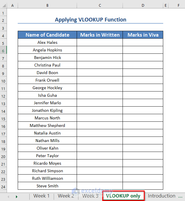
We will search through the three worksheets separately.

We will search lookup_value from one worksheet into a range of cells of another worksheet.

The syntax of the formula will be:

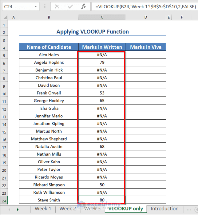
=VLOOKUP(lookup_value,‘Sheet_name’!table_array, col_index_number,FALSE)

To search for the Marks in Written of the Candidates for Week 1, enter this formula in the C5 cell of the new worksheet:

=VLOOKUP(B5,'Week 1'!$B$5:$D$10,2,FALSE)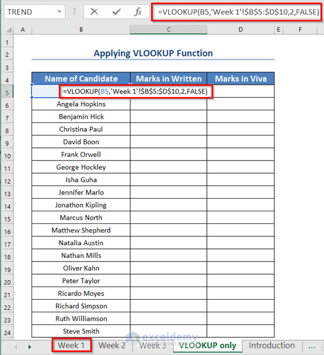

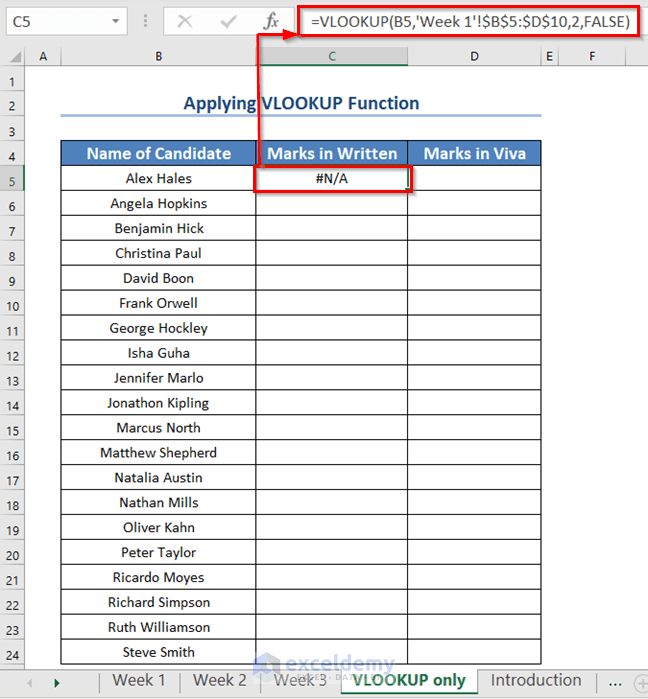
Press ENTER.

You’re seeing an error message (#N/A!) because the name “Alex Hales” in cell B5 of the “VLOOKUP only” sheet isn’t found anywhere in the range B5:D10 of the “Week 1” sheet.

Drag the Fill Handle icon.

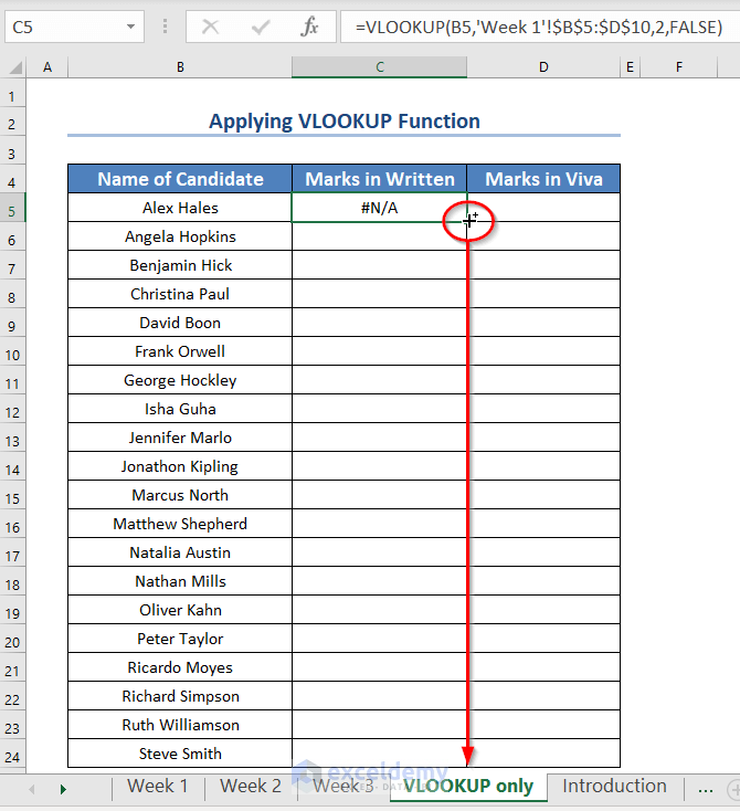
Excel shows the marks of only those candidates who appeared in Week 1, and the rest show errors.

To find the viva mark, enter the following formula in the D5 cell.

=VLOOKUP(B5,'Week 1'!$B$5:$D$10,3,FALSE)

Press ENTER.

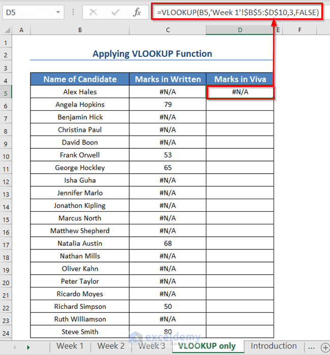
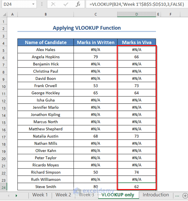
Drag the Fill Handle icon to apply the formula in the rest of the cells.

Excel shows the marks of only those candidates who appeared in Week 1, and the rest show errors.

Notice: We have used relative cell reference for the lookup_value (B5), but absolute cell reference for the table_array ($B$5:$D$10). Because we want the lookup_value to increase one by one while dragging the Fill Handle icon, while the table_array remains constant.

Method 2 – Search on Multiple Sheets with IFERROR Function in Excel

We’ll look for their name in the Week 1 worksheet.
If their name isn’t there, we’ll check the Week 2 worksheet.
Still no luck? We’ll try the Week 3 worksheet.
If their name isn’t on any of these sheets, they must have been absent from the exam.

In the previous section, we learned that VLOOKUP returns N/A! Error if it does not find any match to the lookup_value in the table_array.

To fix this, we’ll nest VLOOKUP functions within the IFERROR function.

The formula will look like:

=IFERROR(VLOOKUP(lookup_value,”Sheet1_Name”!table_array,col_index_number,FALSE),IFERROR(VLOOKUP(lookup_value,”Sheet2_Name”!table_array,col_index_number,FALSE),IFERROR(VLOOKUP(lookup_value,”Sheet3_Name”!table_array,col_index_number,FALSE),”Absent”)))

Enter the following formula in the C5 cell of the “VLOOKUP & IFERROR” sheet.

=IFERROR(VLOOKUP(B5,'Week 1'!$B$5:$D$10,2,FALSE),IFERROR(VLOOKUP(B5, 'Week 2'!$B$5:$D$10,2,FALSE),IFERROR(VLOOKUP(B5,'Week 3'!$B$5:$D$10,2,FALSE),"Absent")))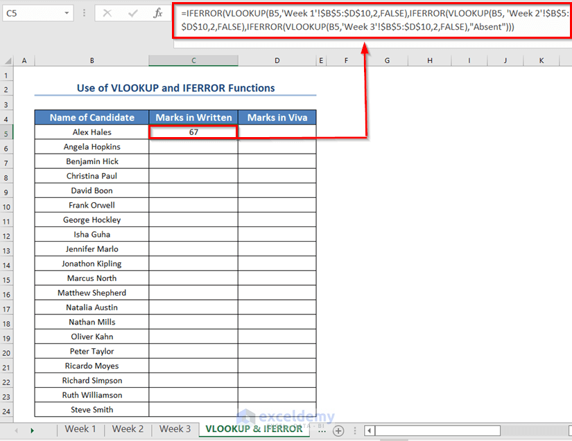

Press ENTER.

You will see the written marks of Alex Hales.

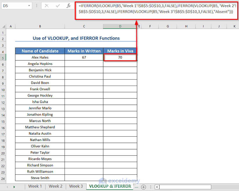
To find the viva marks of Alex Hales, enter the following formula in the D5 cell.

=IFERROR(VLOOKUP(B5,'Week 1'!$B$5:$D$10,3,FALSE),IFERROR(VLOOKUP(B5, 'Week 2'!$B$5:$D$10,3,FALSE),IFERROR(VLOOKUP(B5,'Week 3'!$B$5:$D$10,3,FALSE),"Absent")))

Press ENTER.

Select both cells C5 and D5.
Drag the Fill Handle icon to AutoFill the corresponding data in the rest of the cells C6:D24.

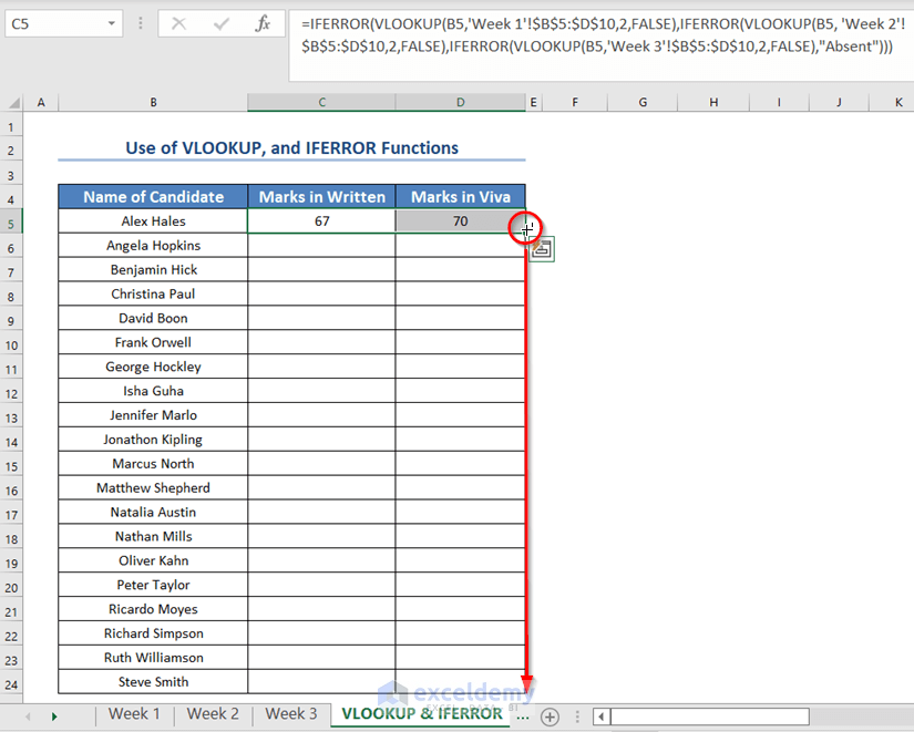
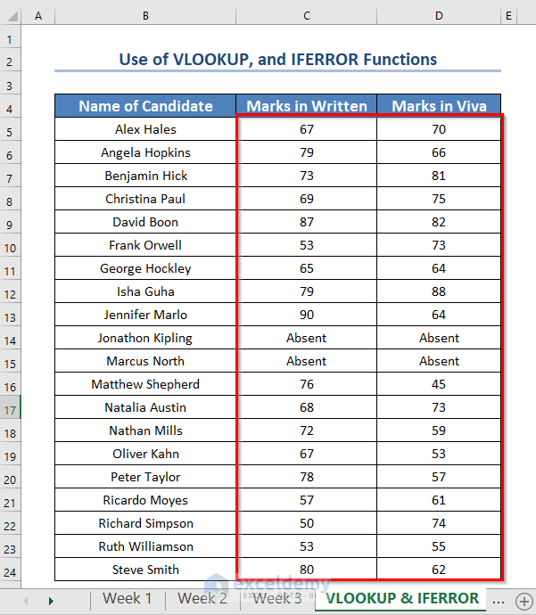
You will see both the marks in written and viva for all the candidates.

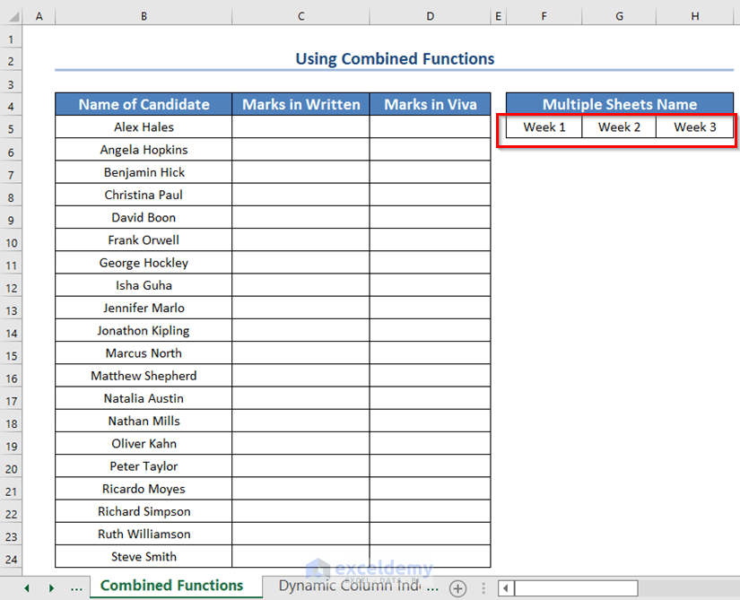
Method 2 – Using Combined Formula to Search on Multiple Sheets in Excel

Create a horizontal array with the names of all the worksheets. We have created one in F5:H5 cells.

Insert the following formula in the C5 cell.

=IFERROR(VLOOKUP(B5,INDIRECT("'"&INDEX($F$5:$H$5,1,MATCH(TRUE,COUNTIF(INDIRECT("'"&$F$5:$H$5&"'!B5:B10"),B5)>0,0))&"'!$B$5:$D$10"),2,FALSE),"Absent")

Press ENTER.

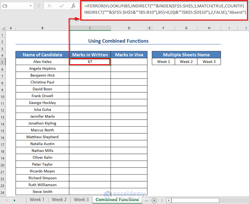
Formula Breakdown

COUNTIF(INDIRECT(“‘”&$F$5:$H$5&”‘!B5:B10”),B5) returns how many times the value in cell B5 is present in the range ‘Week 1′!B5:B10, ‘Week 2’!B5:B10 and ‘Week 3’!B5:B10 respectively. [ $F$5:$H$5 is the names of the worksheets. So the INDIRECT formula receives ‘Sheet_Name’!B5:B10.]
- Output: {0,0,1}.
MATCH(TRUE,{0,0,1}>0,0) returns in which worksheet the value in B5 is present.
- Output: 3.
It returned 3 as the value in B5 (Alex Hales) is in worksheet no 3 (Week 3).
INDEX($F$5:$H$5,1,3) returns the name of the worksheet where the value in cell B5 is.
- Output: “Week 3”.
INDIRECT(“‘”&”Week 3″&”‘!$B$4:$D$9”) returns the total range of cells of the worksheet in which the value in B5 is present.
- Output: {“Nathan Mills”,72,59;”Ruth Williamson”,53,55;”Alex Hales”,67,70;”Matthew Shepherd”,76,45;”Christina Paul”,69,75;”Ricardo Moyes”,57,61}.
VLOOKUP(B5,{“Nathan Mills”,72,59;”Ruth Williamson”,53,55;”Alex Hales”,67,70;”Matthew Shepherd”,76,45;”Christina Paul”,69,75;”Ricardo Moyes”,57,61},2,FALSE) returns the 2nd column of the row from that range where the value in cell B5 matches.
- Output: 67.
And in case the name is not found in any worksheet, it will return “Absent” because we nested it within an IFERROR function.

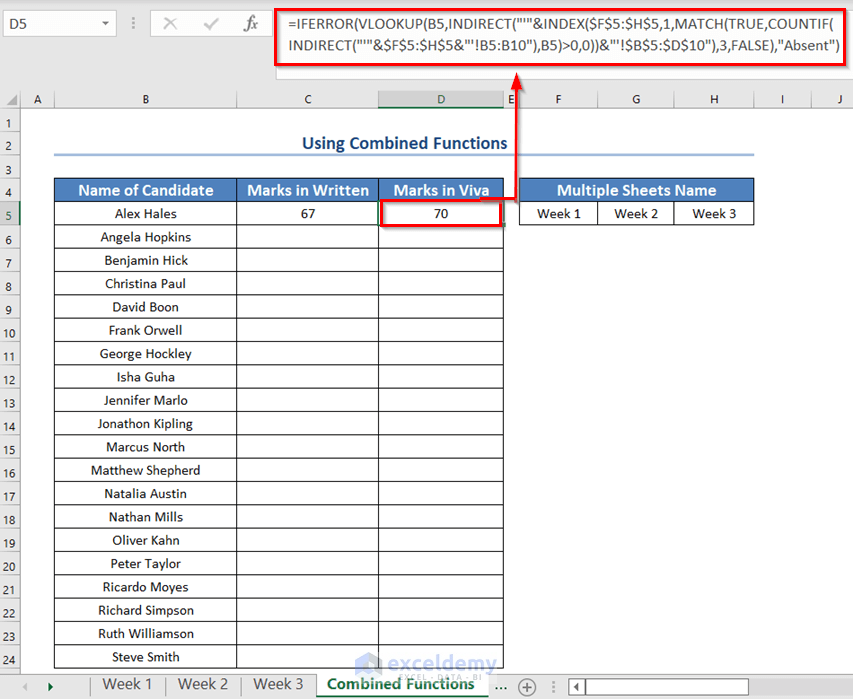
You can use a similar formula to find out the Viva marks of the candidates.

Change the col_index_number from 2 to 3 and enter the formula.

=IFERROR(VLOOKUP(B5,INDIRECT("'"&INDEX($F$5:$H$5,1,MATCH(TRUE,COUNTIF(INDIRECT("'"&$F$5:$H$5&"'!B5:B10"),B5)>0,0))&"'!$B$5:$D$10"),3,FALSE),"Absent")

Press ENTER to get the result.

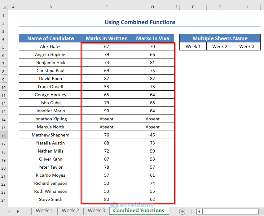
Drag the Fill Handle icon.

We will get both the written and viva marks of all the candidates. Names that are not found will be marked as absent.

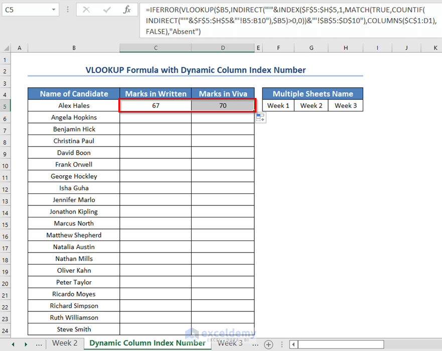
Method 2 – VLOOKUP Formula with Dynamic Column Index Number

Insert the following formula in the C5 cell.

=IFERROR(VLOOKUP($B5,INDIRECT("'"&INDEX($F$5:$H$5,1,MATCH(TRUE,COUNTIF(INDIRECT("'"&$F$5:$H$5&"'!B5:B10"),$B5)>0,0))&"'!$B$5:$D$10"),COLUMNS($C$1:D1),FALSE),"Absent")

Press ENTER.

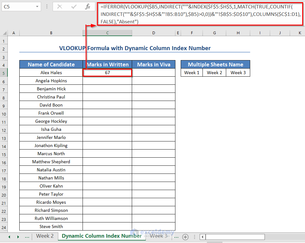
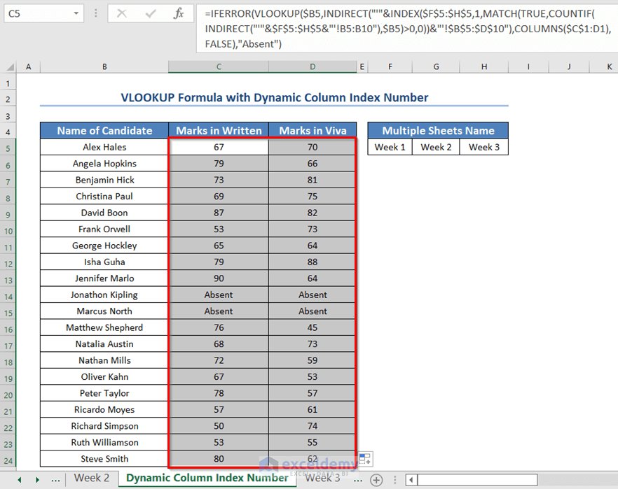
Drag the Fill Handle icon to the right side to get the Viva marks.

Drag the Fill Handle icon down.

You will see both the marks in written and viva for all the candidates.

Notice: We have changed the lookup_value from B5 to $B5, so that it remains unchanged when dragging to the right, but changes when dragging down.

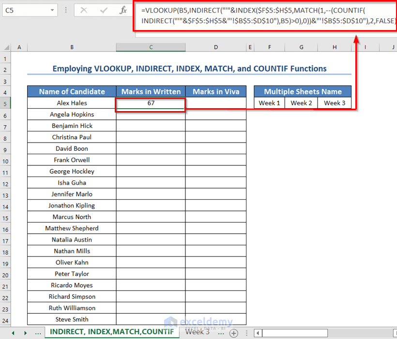
Method 5 – VLOOKUP Formula with Combined Functions in Excel

Steps:

Select a new cell C5 where you want to keep the written marks.
Use the formula given below in the C5 cell.

=VLOOKUP(B5,INDIRECT("'"&INDEX($F$5:$H$5,MATCH(1,--(COUNTIF(INDIRECT("'"&$F$5:$H$5&"'!$B$5:$D$10"),B5)>0),0))&"'!$B$5:$D$10"),2,FALSE)

Press ENTER.

Use the following formula in the D5 cell to get the Viva marks.

=VLOOKUP(B5,INDIRECT("'"&INDEX($F$5:$H$5,MATCH(1,--(COUNTIF(INDIRECT("'"&$F$5:$H$5&"'!$B$5:$D$10"),B5)>0),0))&"'!$B$5:$D$10"),3,FALSE)

Press ENTER.

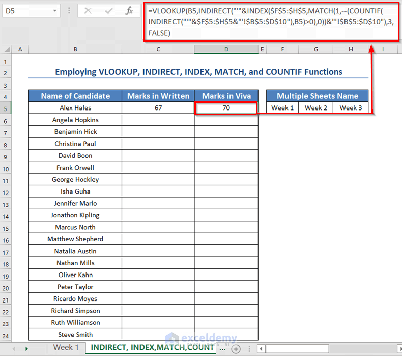
Drag the Fill Handle icon.

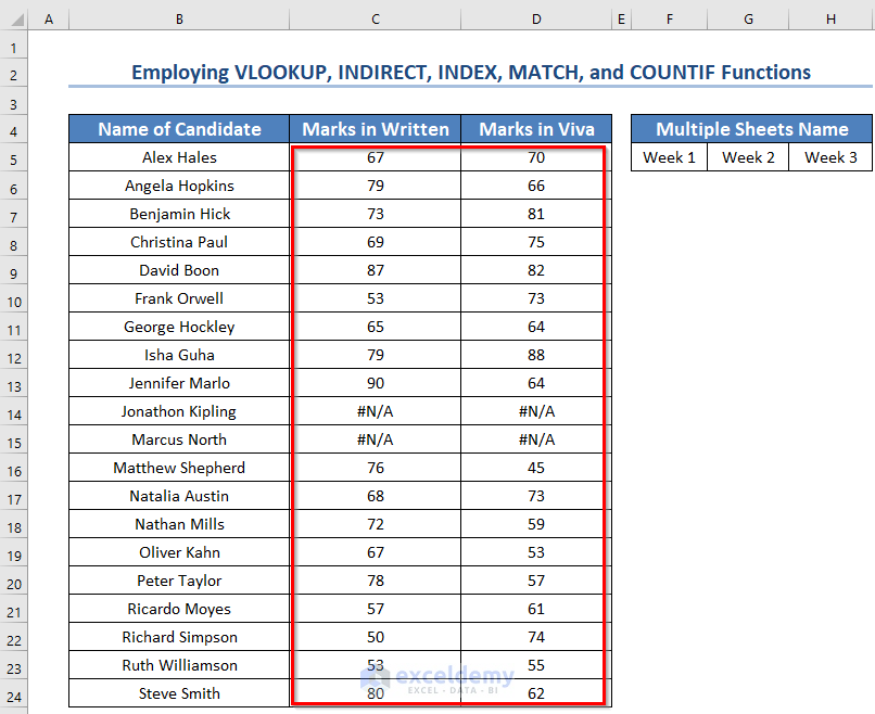
You will see both the written and viva marks of all the candidates. It will show #N/A error where the names were missing in the mentioned sheets.

Limitations of VLOOKUP Function and Some Alternatives in Excel

You cannot use the VLOOKUP function when the lookup_value is not in the first column of the table. For example, in the previous example, you cannot use the VLOOKUP function to know the name of the candidate who got a 90 on the written exam.
You can use the IF, IFS, INDEX MATCH, XLOOKUP, or FILTER functions of Excel to solve this (check this article for more details).
VLOOKUP returns only the first value if more than one value matches the lookup_value. In such cases, you can use the FILTER function to get all the values (Check this article to learn more).