Excel FILTER Function: Overview
We have the years, the host countries, the champion countries, and the runners-up countries of all the FIFA World Cups in columns B, C, D, and E, respectively.
Let’s get the years when Brazil became the champion.
The FILTER function takes three arguments: a range of cells called an array, a criterion called include, and a value called if_empty that is returned in case the condition is not met for any cell. The resulting syntax is:
=FILTER(array,include,[if_empty])One of the formulas you can use to get the years when Brazil was the champion is:
=FILTER(B5:B25,D5:D25="Brazil","")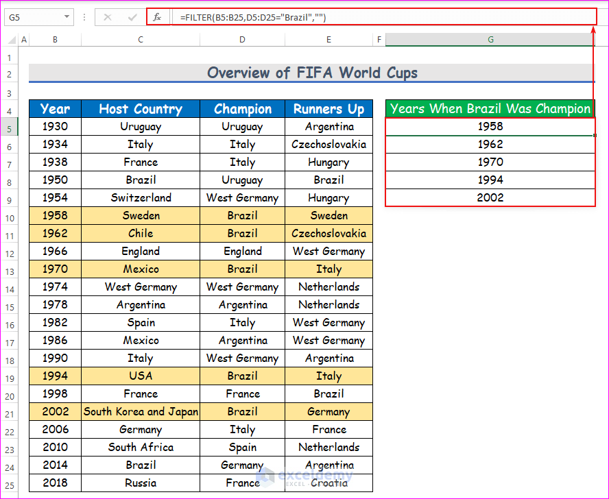
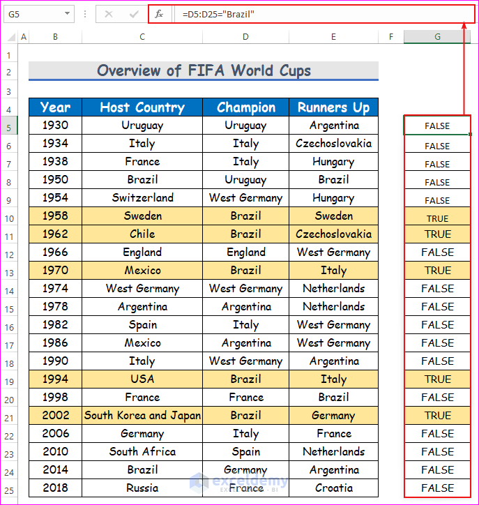
D5:D25=”Brazil” goes through all the cells from D5 to D25 and returns a TRUE if it finds Brazil. If not, the result is FALSE, and the function ignores the cell.
The formula FILTER(B5:B25,D5:D25=”Brazil”,””) then becomes
=FILTER({B5,B6,B7,...,B25},{FALSE,FALSE,...,TRUE,...,FALSE},"")For each TRUE value, FILTER returns the corresponding cell from the array {B5,B6,B7,…,B25}
We get TRUE only for the cells B9, B10, B12, B18, and B20. So, it returns only the contents of these cells, 1958, 1962, 1970, 1994, and 2002.
These are the years when Brazil became the champion.
As another example, here’s a formula for determining when the host country was the champion:
=FILTER(B5:B25,C5:C25=D5:D25,””)
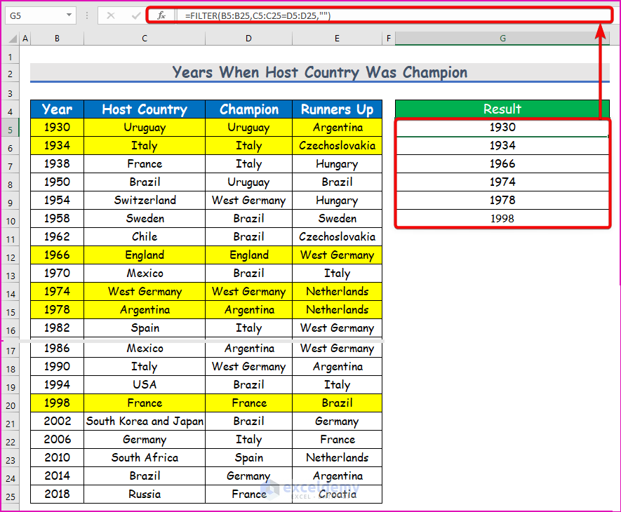
The host country became champion in 1930, 1934, 1966, 1974, 1978, and 1998.
We’ll use the same dataset to apply multiple criteria in the FILTER function.
Method 1 – Using the FILTER Function with Multiple OR Criteria
Let’s filter out all the years when Italy was the host or the champion, or both. This is an OR-type multiple criteria.
Steps:
- Select cell G5 and insert the following formula, then hit Enter.
=FILTER(B5:B25,(C5:C25="Italy")+(D5:D25="Italy"))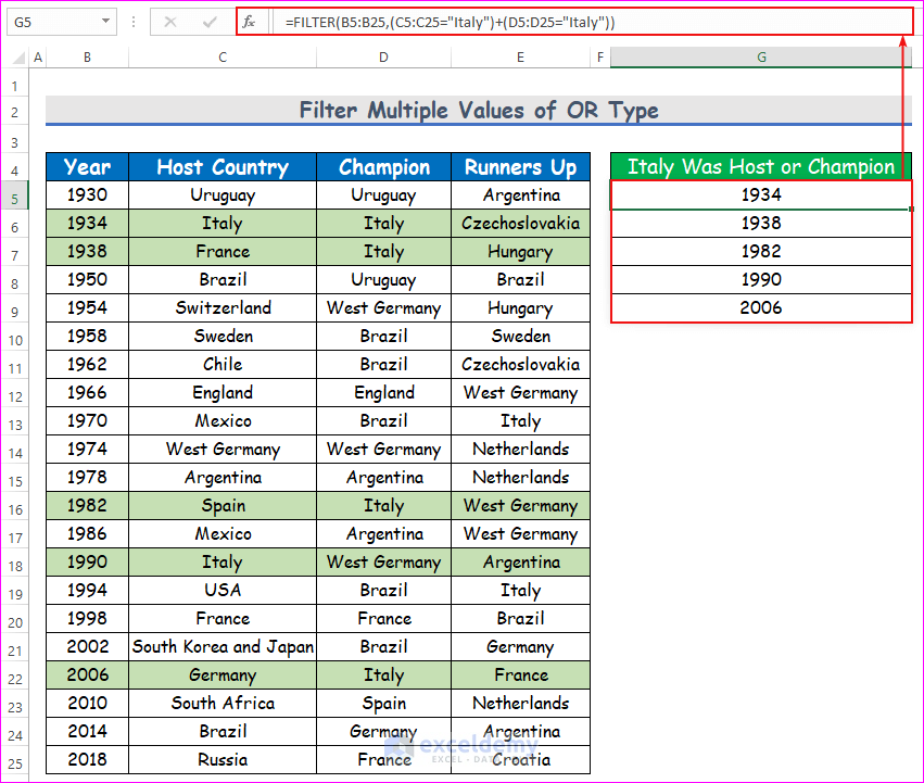
Italy was either the host or champion or both in the years 1934, 1938, 1982, 1990, and 2006.
Formula Breakdown
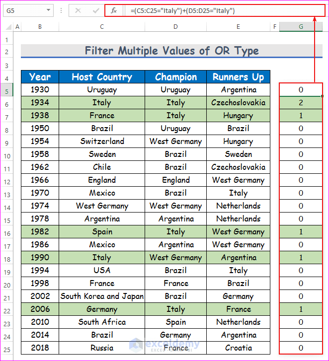
- C5:C25=”Italy” returns an array of TRUE or FALSE. TRUE when Italy was the host, or FALSE otherwise.
- D5:D25=”Italy” also returns an array of TRUE or FALSE. TRUE when Italy was the champion, or FALSE otherwise.
- (C5:C25=”Italy”)+(D5:D25=”Italy”) adds two arrays of Boolean values, TRUE and FALSE. It considers each TRUE as a 1, and each FALSE as a 0.
- So it returns a 2 when both criteria are satisfied, a 1 when only one criterion is satisfied, and a 0 when no criterion is satisfied.
- The FILTER formula returns a result if the condition is more than 0, so it will work for one or more positive results for the row.
Here’s the formula for determining when Brazil became the champion or Italy became the runner-up:
=FILTER(B5:B25,(D5:D25="Brazil")+(E5:E25="Italy"))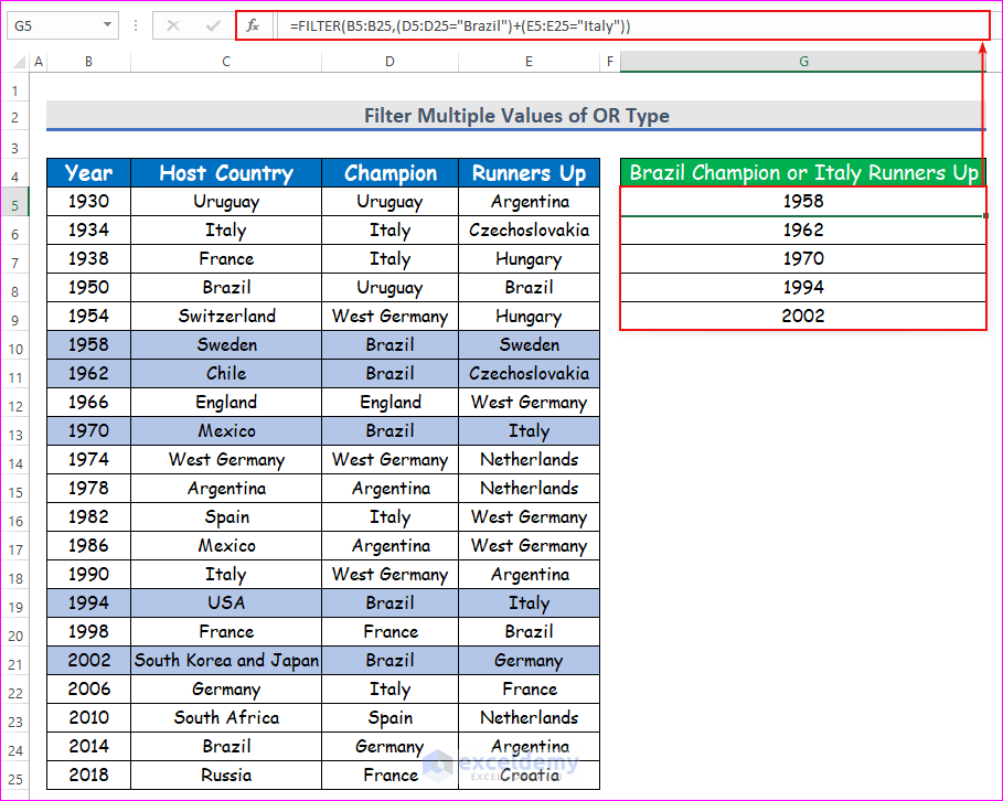
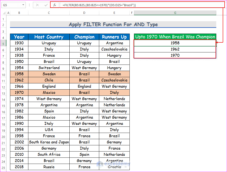
Method 2 – Applying the FILTER Function with Multiple AND-Type Criteria
Up until 1970, the FIFA World Cup was called the “Jules Rimet” trophy. After 1970, it was renamed the FIFA World Cup. What are the years when Brazil won the “Jules Rimet” trophy?
There are two criteria here:
- The year must be less than or equal to 1970.
- The champion country has to be Brazil.
This is an AND-type condition, where both have to be met simultaneously.
Steps:
- Select cell G5 and insert the following formula, then hit Enter.
=FILTER(B5:B25,(B5:B25<=1970)*(D5:D25="Brazil"))Formula Breakdown
(B5:B25<=1970returns a TRUE if the year is less than or equal to 1970, otherwise FALSE.(D5:D25="Brazil")returns a TRUE if the champion country is Brazil, otherwise FALSE.(B5:B25<=1970)*(D5:D25="Brazil")multiplies two arrays of TRUE and FALSE, but considers each TRUE as 1 and each FALSE as 0.- The * operator returns a 1 if both the criteria are met, otherwise it returns a 0.
- Now the formula becomes:
=FILTER({B4,B5,B6,...,B24},{0,0,...,1,1,...,0}) - It returns the year in column B when it faces a 1 and returns no result when it faces a 0.
Here’s the formula to look up the years before 2000 when Brazil was the champion and Italy was the runner-up:
=FILTER(B5:B25,(B5:B25<2000)*(D5:D25="Brazil")*(E5:E25="Italy"))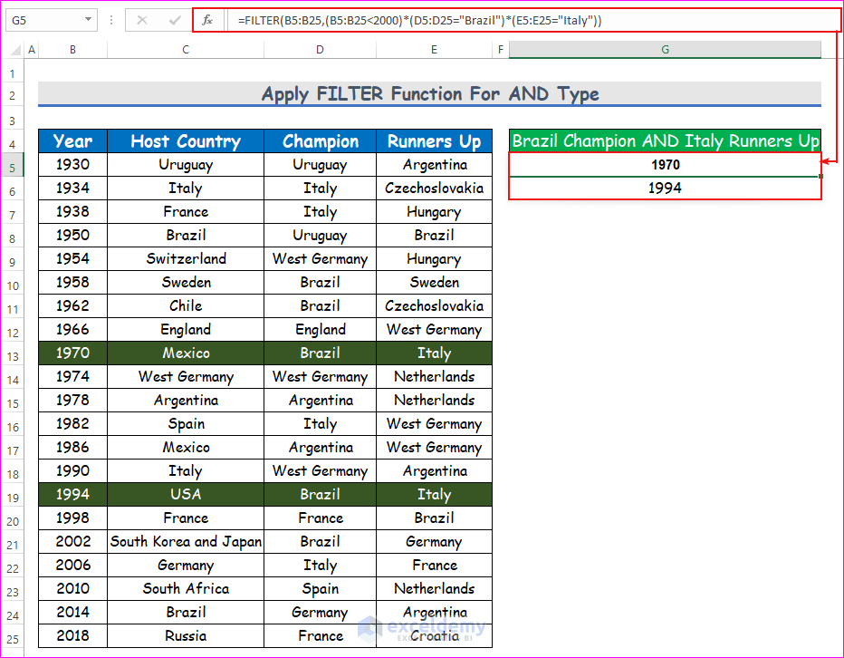
Method 3 – Filtering Multiple Criteria by Combining AND and OR Conditions in Excel
Case 1 – OR within OR
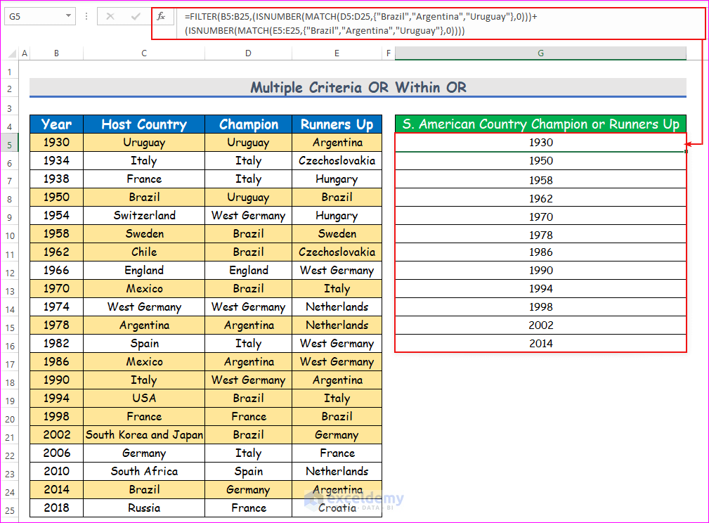
Let’s find the years when a South American country (Brazil, Argentina, or Uruguay) was either a champion or a runner-up.
Steps:
- Select cell G5 and insert the following formula, then hit Enter.
=FILTER(B5:B25,(ISNUMBER(MATCH(D5:D25,{"Brazil","Argentina","Uruguay"},0)))+ (ISNUMBER(MATCH(E5:E25,{"Brazil","Argentina","Uruguay"},0))))Formula Breakdown
MATCH(D4:D24,{"Brazil","Argentina","Uruguay"},0)returns 1 if the champion team is Brazil, 2 if the champion team is Argentina, 3 if the champion team is Uruguay, and an error (N/A) if the champion team is none of them.ISNUMBER(MATCH(D4:D24,{"Brazil","Argentina","Uruguay"},0))converts the numbers into TRUE and the errors into FALSE.ISNUMBER(MATCH(E4:E24,{"Brazil","Argentina","Uruguay"},0))returns a TRUE if the runners-up country is either Brazil, Argentina or Uruguay. And FALSE(ISNUMBER(MATCH(D4:D24,{"Brazil","Argentina","Uruguay"},0)))+(ISNUMBER(MATCH(E4:E24,{"Brazil","Argentina","Uruguay"},0)))returns a 1 or 2 if either a South American country is champion, or runners up, or both.- The formula becomes:
=FILTER({B4,B5,...,B24},{2,0,0,2,...,1,0})
- It returns a year from column B if it finds a number greater than zero, and returns no result otherwise.
Case 2 – OR within AND
Let’s determine the years when both the champion and runner-up were from South America (Brazil, Argentina, or Uruguay).
- Select cell G5 and insert the following formula, then hit Enter.
=FILTER(B4:B24,(ISNUMBER(MATCH(D4:D24,{"Brazil","Argentina","Uruguay"},0)))*(ISNUMBER(MATCH(E4:E24,{"Brazil","Argentina","Uruguay"},0))))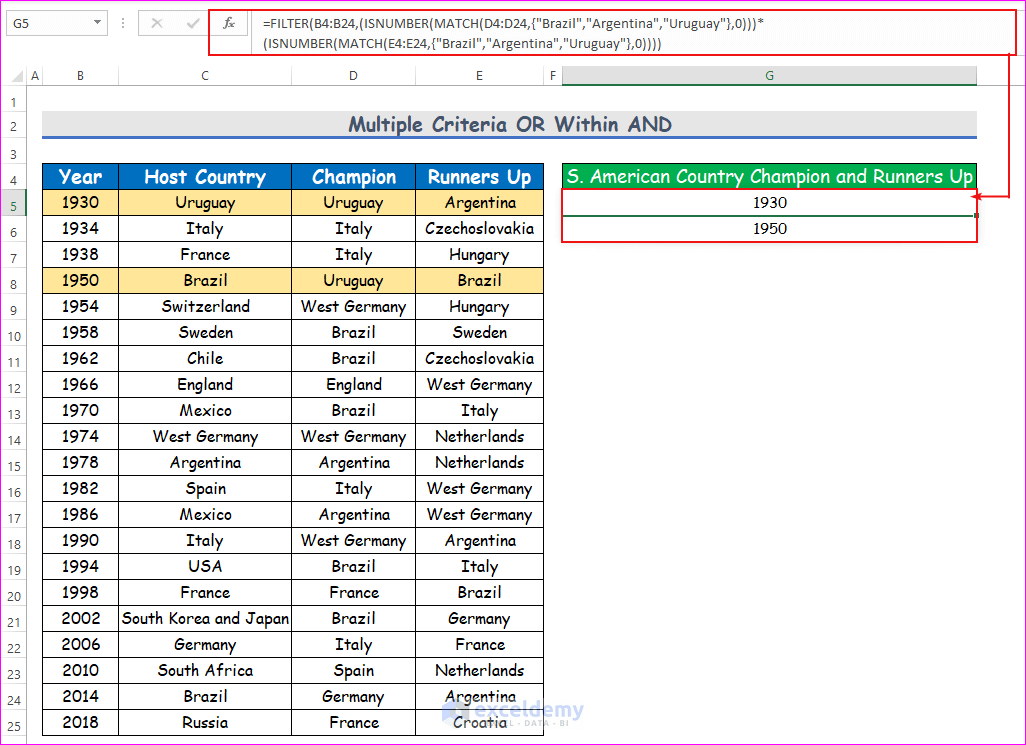
Method 4 – Inserting the FILTER Function in Multiple Columns
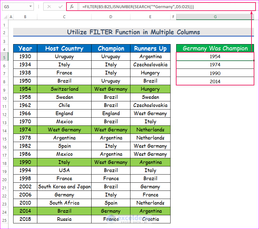
Let’s identify the years when Germany was the champion. Before 1990, the country that participated was West Germany, so we’ll count it as well.
- Select cell G5 and insert the following formula, then hit Enter.
=FILTER(B5:B25,ISNUMBER(SEARCH("*Germany",D5:D25)))Formula Breakdown
SEARCH("*Germany",D5:D25)searches for anything having Germany in the end in the array D5 to D25. If you need Germany in the middle, use “*Germany*”.- It returns a 1 if it finds a match (West Germany and Germany) and returns an Error
ISNUMBER(SEARCH("*Germany",D5:D25))converts the 1’s into TRUE, and the errors into FALSE.- Finally,
FILTER(B5:B25,ISNUMBER(SEARCH("*Germany",D5:D25)))returns the years from column B when it faces a TRUE, otherwise returns no result.
Let’s see when the FIFA World Cup was hosted by two countries. For this, the table contains ” and “ in the host country name.
- Select cell G5 and insert the following formula, then hit Enter.
=FILTER(B5:B25,ISNUMBER(SEARCH("* and *",C5:C25)))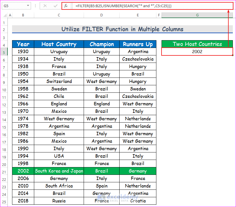
Alternative Options to Filter Multiple Criteria in Excel
The FILTER function is available only for Office 365. Here are some alternatives:
- To find the years when Italy was the host country or champion, use the below formula:
=IF((C5:C25="Italy")+(D5:D25="Italy"),B4:B24,"")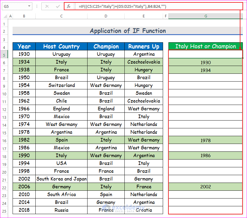
- To find the years when Brazil was champion up to 1970, use this formula:
=IF((B5:B25<=1970)*(D5:D25="Brazil"),B5:B25,"")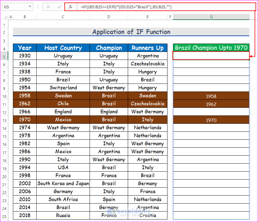
Note: You can not have the blank cells removed like the FILTER function in this way. And press Ctrl + Shift + Enter to enter the formulas.
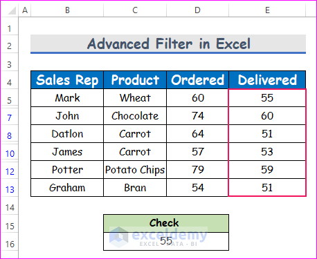
How to Use the Advanced Filter in Excel
We’ll apply multiple criteria on one column using calculated data. We’re going to find delivered products with quantity more than 50 but less than 100.
- Apply the following formula:
=IF(AND(E5<100,E5>50),E5,FALSE)The output in cell C16 is 55 as the delivered quantity falls in the range.
- Select the Advanced command under the Sort & Filter options from the Data tab.
- Put the whole dataset as the List range and cells C15:C16 as the Criteria range.
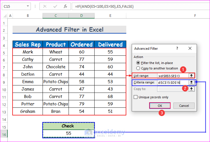
- Hit OK to see the result, i.e., a list of delivered products having a quantity in the range from 50 to 100.
Download the Practice Workbook
<< Go Back to Filter in Excel | Learn Excel
Get FREE Advanced Excel Exercises with Solutions!

Sir, 28th July,2021.
I am impressed by the example given by you,i.e. Filter Function.
Hope to receive more functions in future too.
Thanking you.
Kanhaiyalal Newaskar.
This is great!
Thanks
M