Excel AutoFilter – A Complete Guide

This is an overview.

Download Practice Workbook

Download this file to practice.

How to Enable the AutoFilter in an Excel Dataset

1. Apply the Filter in the Home Tab

• Select any cell inside your range. Here, F7.
• In Editing, select Sort & Filter.
• Choose Filter.

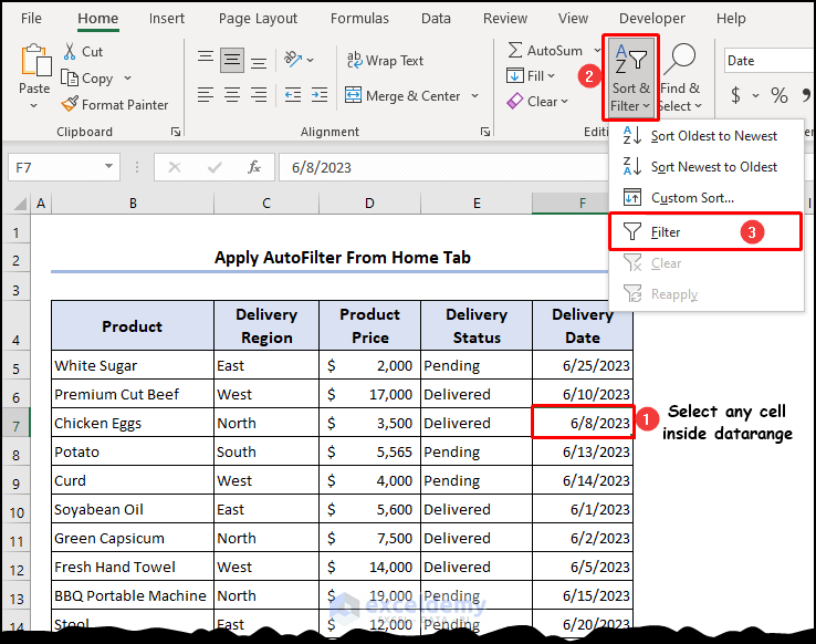
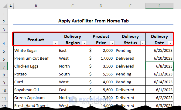
You can see the Filter buttons in the header column.

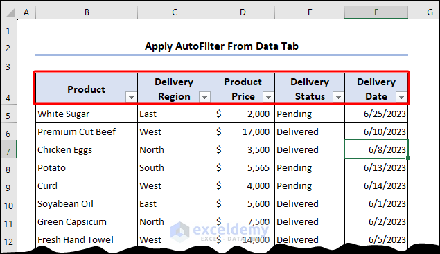
2. Apply the Filter in the Data Tab

• Select any cell inside your range. Here, F7.
• In Sort & FIlter, select Filter.

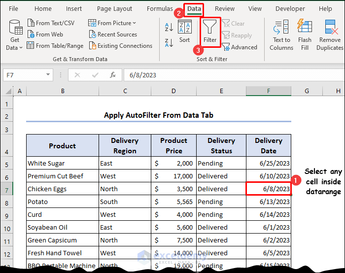
You can see the Filter buttons in the header column.

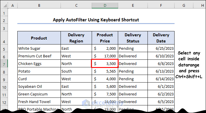
3. Use a Keyboard Shortcut to Enable the Filter

• Select D7.
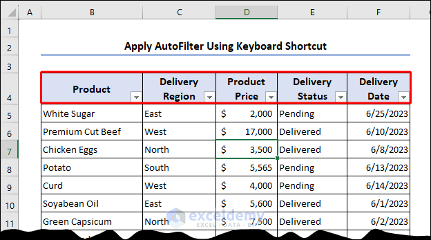
• Press Ctrl + Shift + L to apply the filter.

You can see the Filter buttons in the header column.

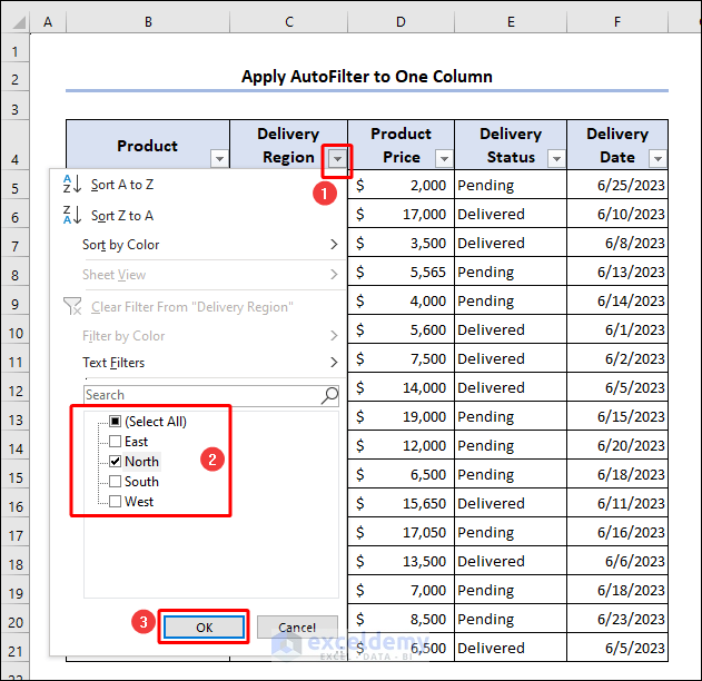
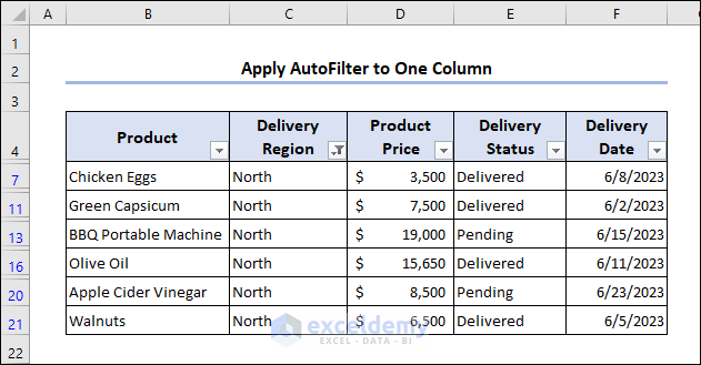
How to Apply AutoFilter to One Column/Criteria in Excel

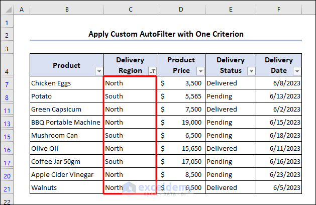
To see the product details of products delivered in the North region:

• Click the Filter button beside Delivery Region.
• Check North and press OK.

This is the output.

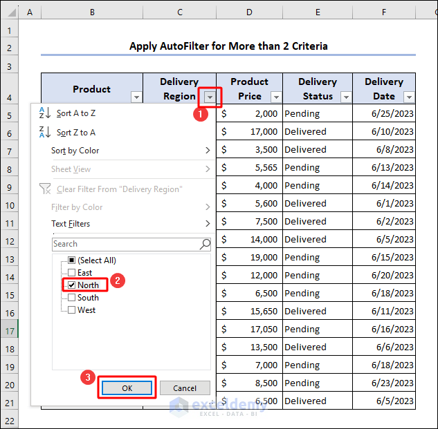
How to Apply AutoFilter with Two or More Criteria in Excel

To see product details with the following criteria:

1. Delivery region: North,
2. Delivered value over $6000,
3. Delivery status: Delivered.

• Click the Filter button beside Delivery Region.
• Select North and click OK.

• Click the Filter button beside Product Price.
• In Number Filters, select Greater Than.

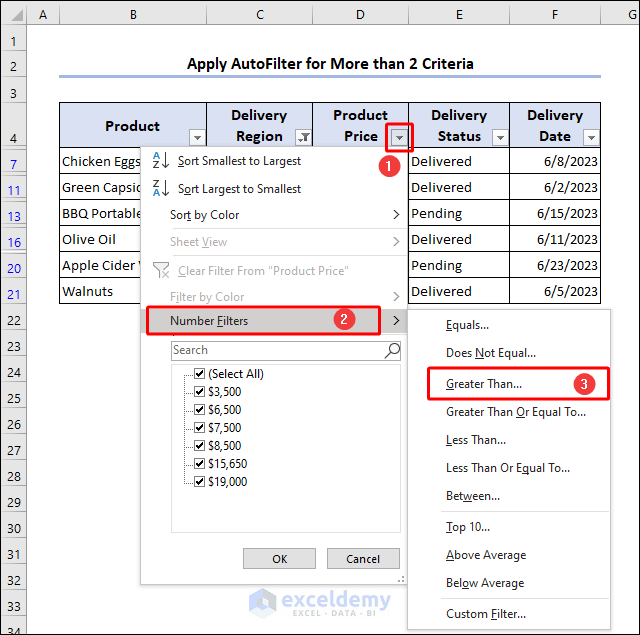
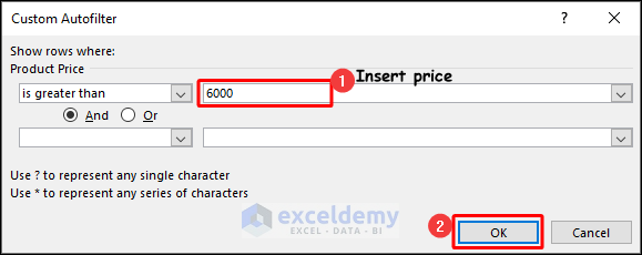
• In the Custom AutoFilter dialog box, enter the number: 6000.
• Click OK.

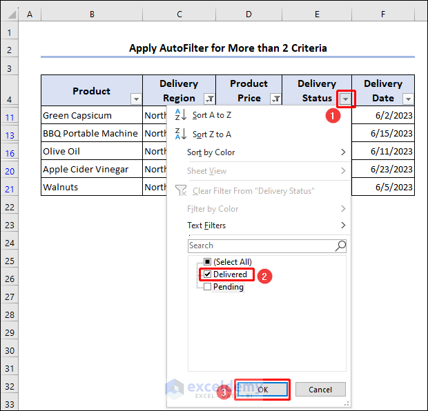
• To filter the delivery status, click the Filter button beside Delivery Status.
• Uncheck Pending and click OK.

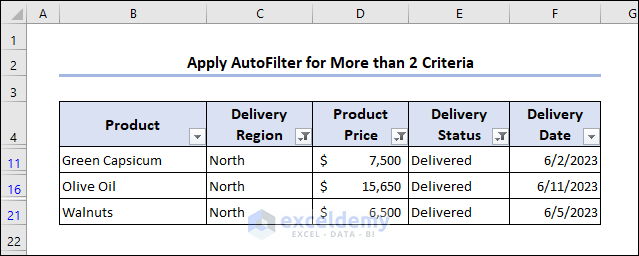
This is the output.

How to Filter the Highest and Lowest Values in Excel

1. AutoFilter the Highest Values

• Click the Filter button next to Product Price.
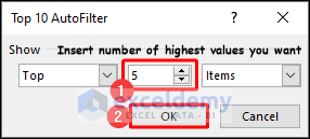
• In Number Filters, select Top 10.

• In the middle box, choose the number of highest values:5.
• Click OK.

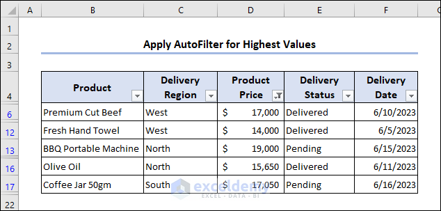
You will see the 5 highest valued products.

2. AutoFilter the Lowest Values

• Click the Filter button next to Product Price.
• In Number Filters, select Top 10.

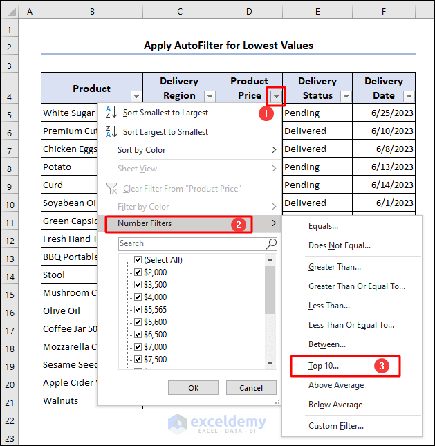
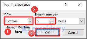
• In the left box, choose Bottom to get the lowest prices.
• In the middle box, choose the number of lowest values: 5 here.
• Click OK.

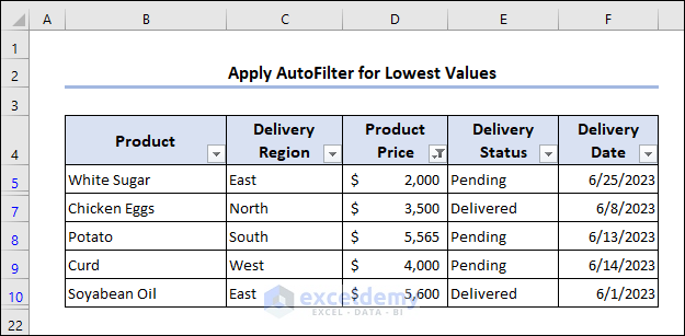
You will see the 5 lowest valued products.

How to Filter by Color in Excel

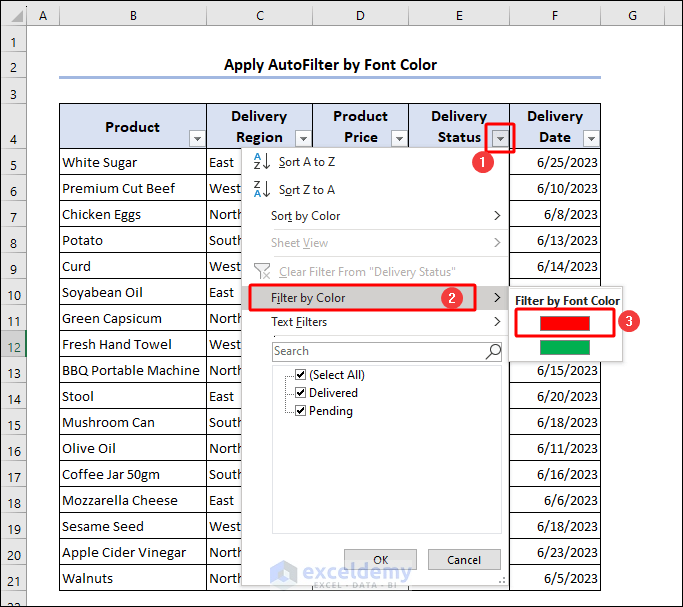
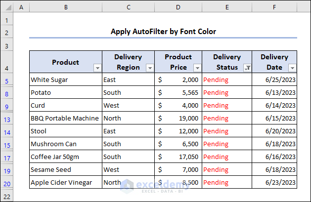
1. Filter by Font Color

Set the font color of Pending as red and Delivered as green.

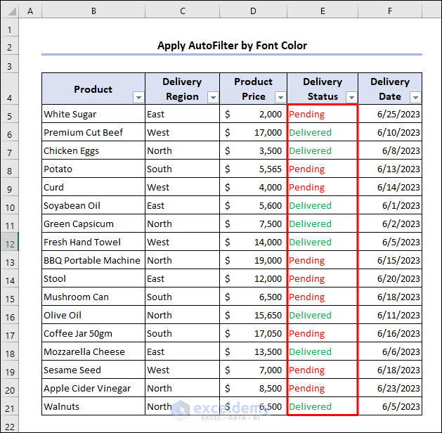
• Click the Filter button next to Delivery Status.
• Choose Filter by Color and select red to see the Pending items.

The Pending items are filtered.

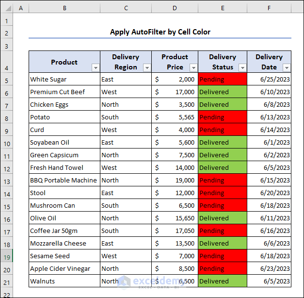
2. Filter by Cell Color

The cells with Pending status are colored red and Delivered are colored green.

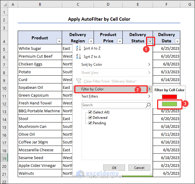
• Click the Filter button next to Delivery Status.
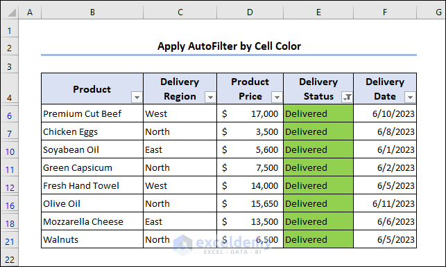
• Choose Filter by Color and select green to see the Delivered items.

The Delivered items are filtered.

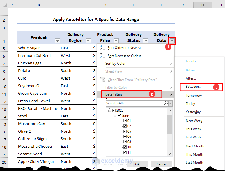
How to Filter a Specific Date Range in Excel

To see the product lists that are delivered or will be delivered between 10 June 2023 to 15 June 2023.

• Click the Filter button next to Delivery Date.
• In Date Filters, select Between.

• Enter the dates in the Custom Autofilter dialog box and click OK.

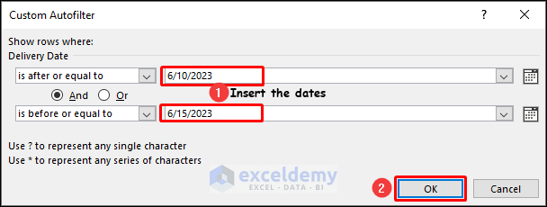
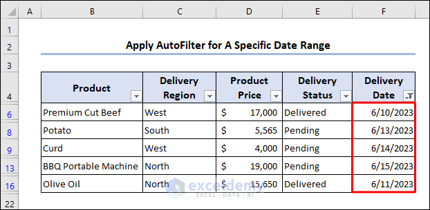
• You will find the products listed for delivery within those dates.

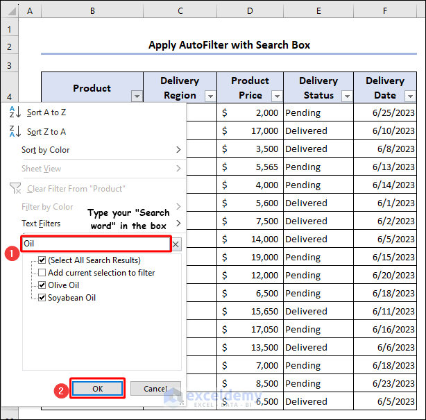
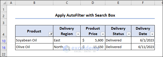
How to Use the AutoFilter with a Search Box in Excel

We want to find the product’s name with the word Oil.

• Click the Filter button next to Product.
• In the Search Box, enter Oil and click OK.

Products with the word Oil are filtered.

How to Filter Blank Cells in Excel

There are two blank rows in the dataset.

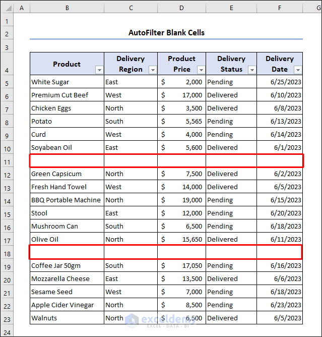
• Click the Filter button next to Delivery Region.
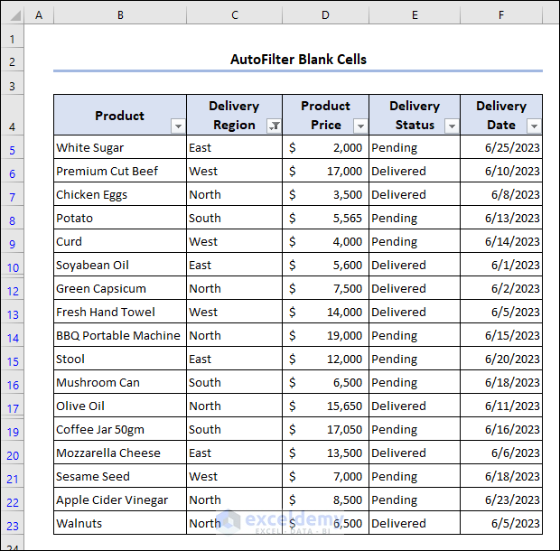
• Uncheck Blanks and click OK.

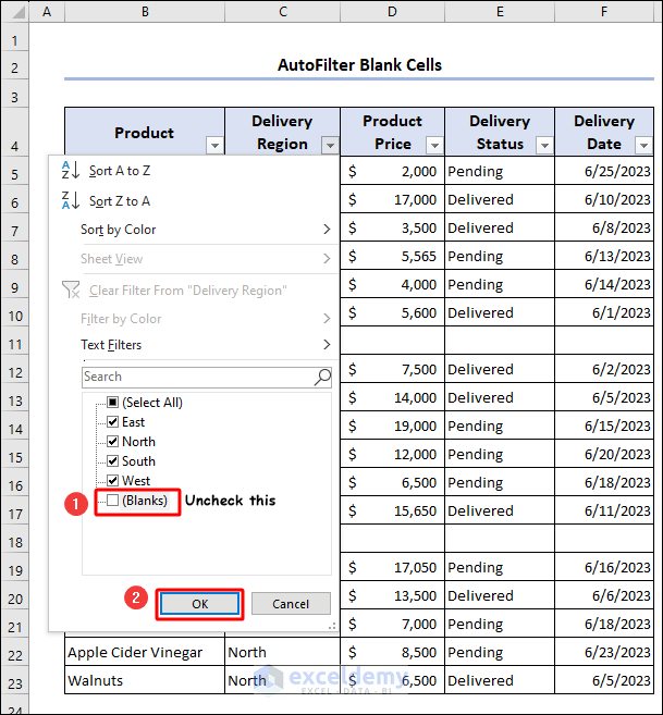
Blank rows are hidden.

How to Use a Custom AutoFilter in Excel

1. Filter for One Criterion

To see the region names with th at the end.

• Click the Filter button next to Delivery Region.
• In Text Filters, choose Custom Filter.

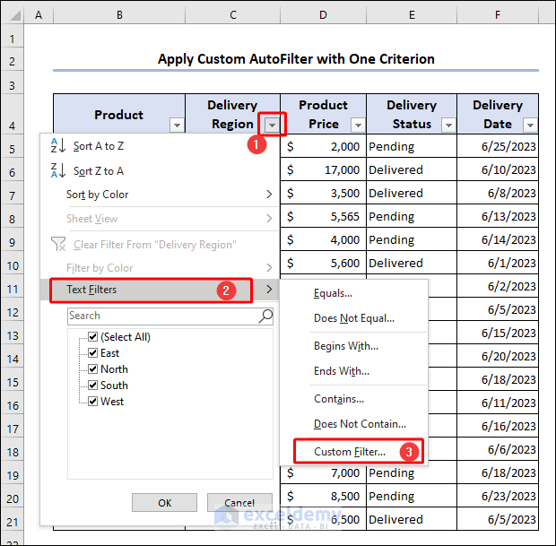
• In Custom Autofilter, choose ends with and enter th in the box.
• Click OK.

North and South are filtered.

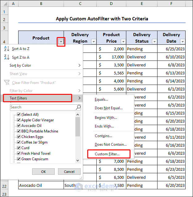
2. Custom Filter for Two Criteria

Use two criteria to filter the dataset:

1. Product name with Oil,

2. Product name with Jar.

• Click the Filter button next to Product.
• In Text Filters, choose Custom Filter.

• In Custom Autofilter, choose contains and enter Oil and Jar in the boxes.
• Check Or.
• Click OK.

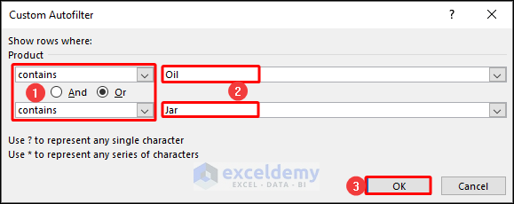
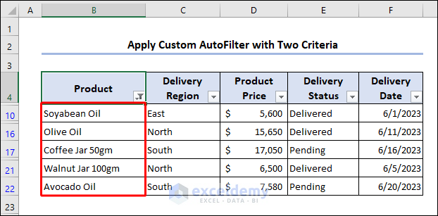
Products with the words Oil or Jar are filtered.

3. Custom Number AutoFilter

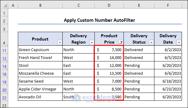
To filter products whose price is greater than $6500 and less than $15000:

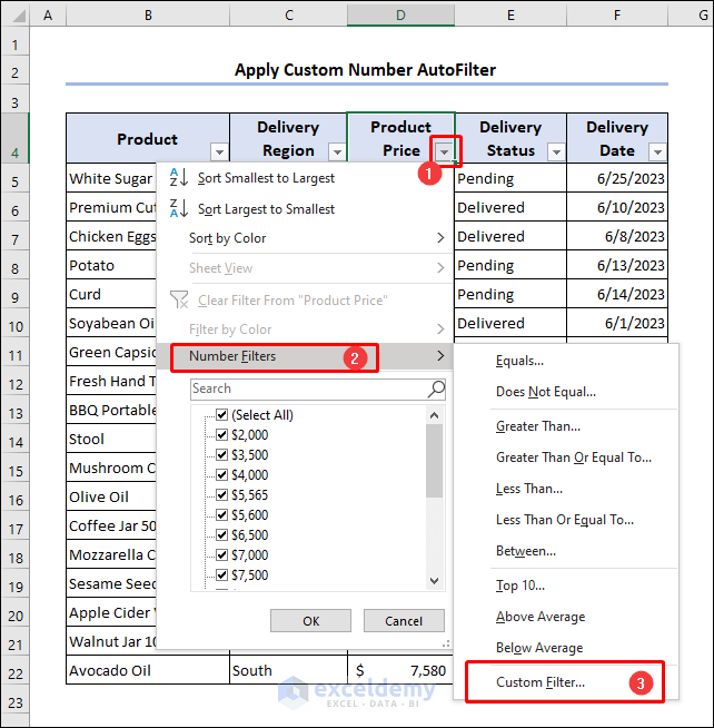
• Click the Filter button next to Product Price.
• In Number Filters, select Custom Filter.

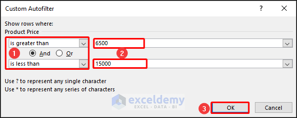
• Choose is greater than and is less than. Enter the upper limit and the lower limit of prices.
• Check And.
• Click OK.

This is the output.

How to Delete Filtered Rows in Excel

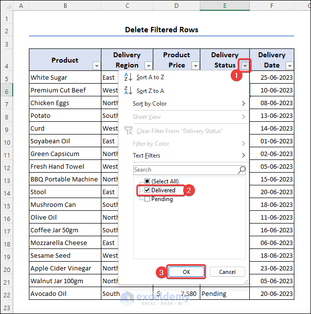
To delete the delivered products from the list.

• Click the Filter button next to Delivery Status.
• Uncheck Pending and check Delivered.
• Click OK.

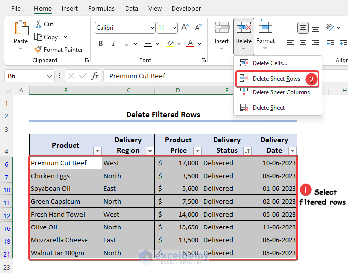
• Select the filtered rows and go to Cells.
• Select Delete Sheet Rows in Delete.

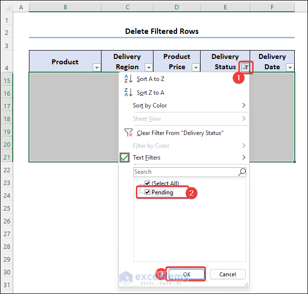
• The delivered items were deleted.
• Click the Filter button and check Pending to show the rest of the rows.

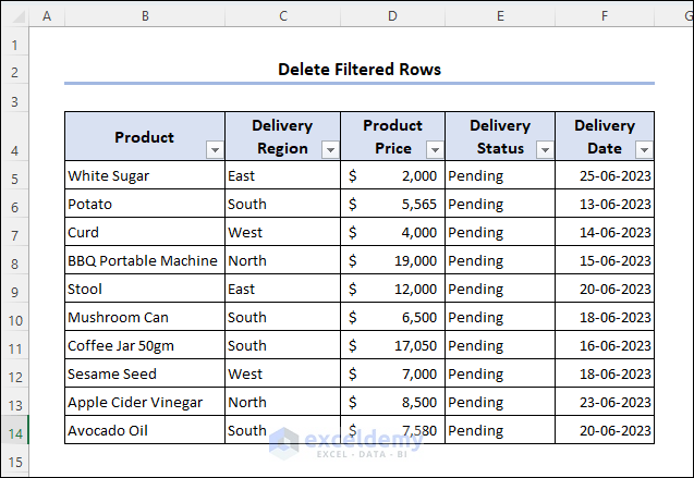
This is the output.

How to Clear AutoFilter in Excel

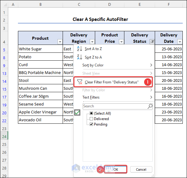
1. Clear A Specific Filter

• Click the Filter button in the Delivery Status.
• Choose Clear Filter from “Delivery Status” and click OK.

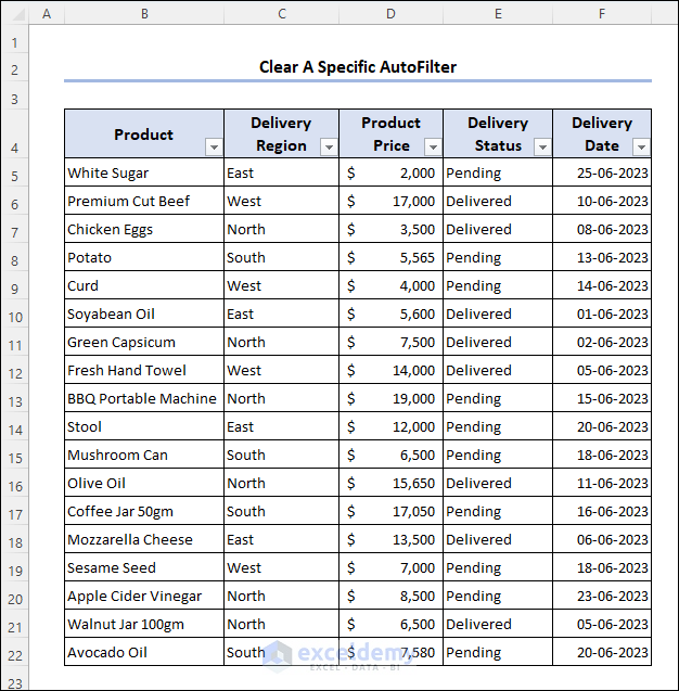
You can see the whole dataset without any filter.

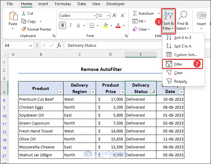
2. Clear All Filters

• To remove all Filters, click the Filter option in Sort & Filter.

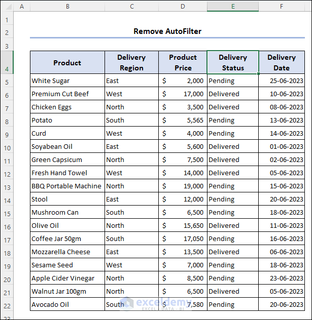
The dataset has no Filter buttons.

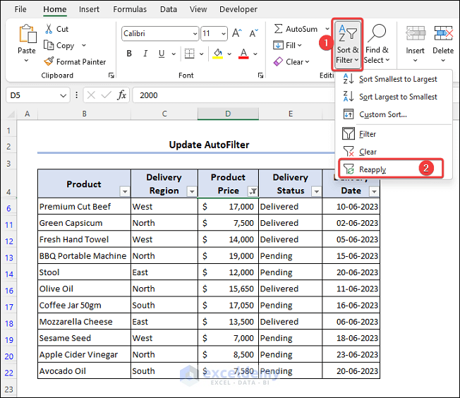
How to Update an AutoFilter

• To update the Filters after adding or removing data, choose Reapply in Sort & Filter.

Frequently Asked Questions

1. Can I use Wildcards with AutoFilter in Excel?

Ans: Yes, use the asterisk (*) as a wildcard to represent any number of characters and the question mark (?) to represent a single character in your filter criteria.

2. Can I filter by text length using AutoFilter in Excel?

Ans: No, you cannot directly filter by text length using AutoFilter in Excel.

3. How do I sort data using the AutoFilter in Excel?

Ans: Select the range you want to sort.

• Go to the Data tab and click the Filter button to enable AutoFilter.
• Click the dropdown arrow in the column header you want to sort.
• Select Sort A to Z (ascending) or Sort Z to A (descending).

Excel AutoFilter: Knowledge Hub

• Use Custom Autofilter in Excel for More Than 2 Criteria

<< Go Back to Filter in Excel | Learn Excel